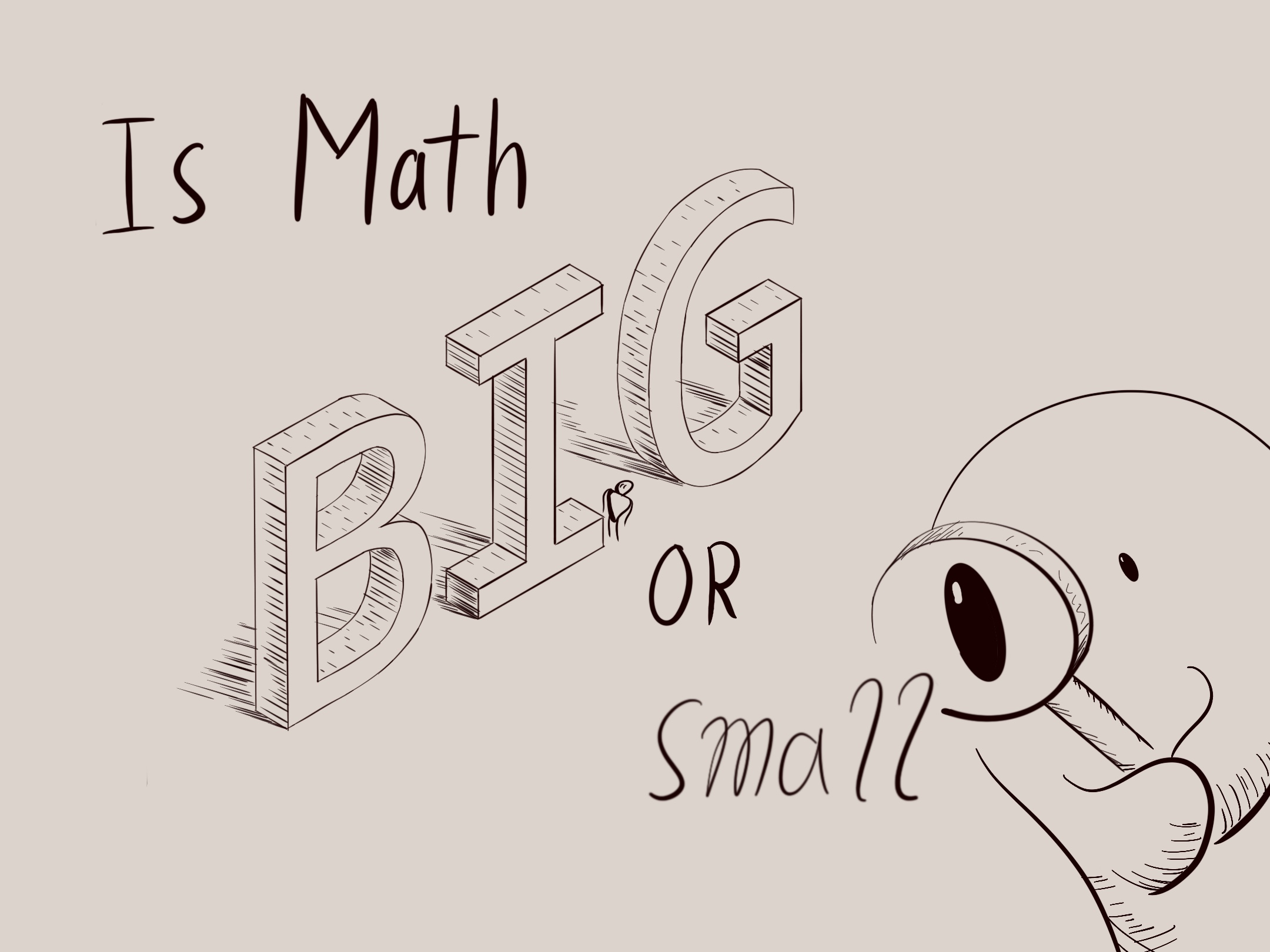
Is math big or small?
Summary:
When Illustrating a mathematical idea, the first thing you need to decide is the scale. Is this concept something you can hold in your hand, or something to wander around in? I will reflect on the scale of various analogies used by research mathematicians, such as Thurston’s train tracks and pictures of symplectic manifolds. Topologists use the metaphors of “geography” and “botany” to organize problems in their field. I will argue that geography and botany are flexible analogies, which give a natural scale for mathematical illustrations.
Presented at:
- Rigorous Illustrations - Their creation and evaluation for mathematical research, IHP trimester on mathematical illustration
🔗 Link to file
The post below is a slightly extended version of my talk at IHP workshop on rigorous illustration. You can also watch the video.
Is math big or small?
Imagine a torus. This is not rhetorical, I want you to summon the mental image of a torus.
- How big is your torus?
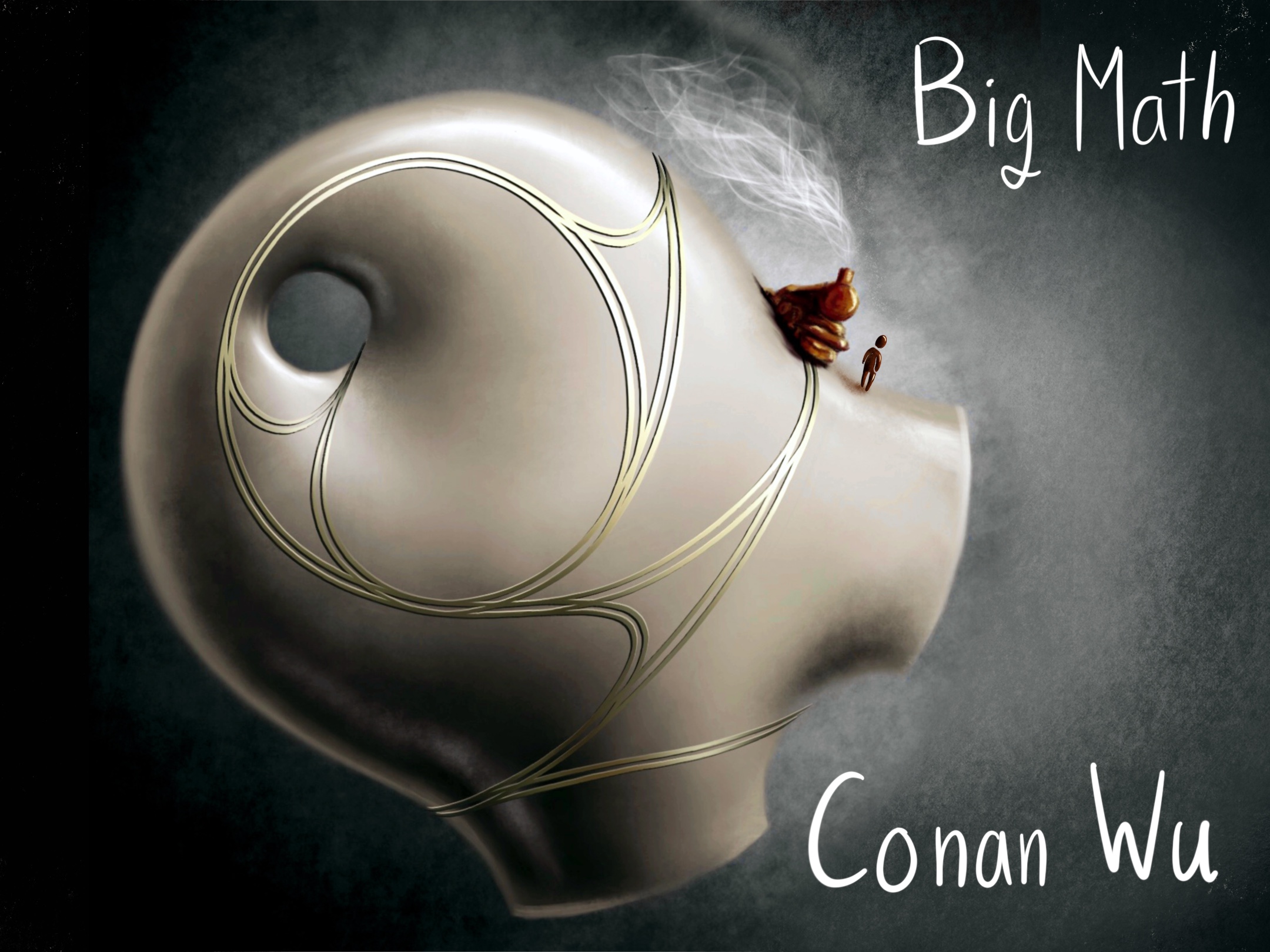
- Why? Ive always struggled with this question. Every time you illustrate a torus, or indeed any mathematical idea, the first thing to decide is the scale. Scale is more than physical size. In this picture, the word “big” feels large because it dwarfs our friend by the I, whereas “small” feels small because its much smaller than the critter analyzing it. Scale is relative to the viewer.
Is math something to hold in your hand, or something to wander around it? To limit our scope, we’ll look at the scale of mathematical imagery used by researchers. I’m interested in those collective hallucinations which are embedded in the way the community conceptualizes mathematical ideas. In this post, we’ll go through several anecdotes of math, big and small, and discuss how the scale effects the illustrations.
Table of contents:
- Train tracks
- Big math in symplectic topology
- Geography and botany, and the isoperimetric island
- Using geography and botany
- Gallery
Train tracks
This story starts in 1971 at UC Berkeley, which had quite a colorful math department. Back then Berkeley students and faculty still held the spirit of 1960’s counterculture. Administration had just constructed a new math building, Evans hall: big, concrete and brutalist. The poster child for ugly college buildings. Here’s a picture:
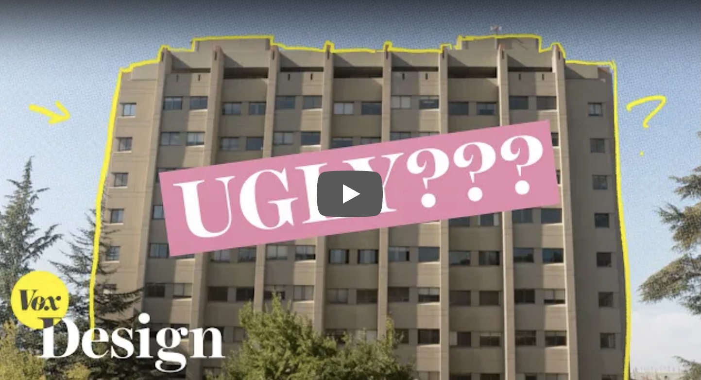
Evans hall
This is a thumbnail for a youtube video about such buildings, with Evans hall front and center. The mathematicians were not pleased about the prospect conducting their creative work in an uninspiring box.
After a rabble rousing talk on fascism and architecture, students and faculty grabbed brushes and paint-cans. They staged a paint-in, covering the windowless hallways with mathematical murals. A young grad student named Bill Thurston approached topologist Dennis Sullivan with a sketch from his notebook, and asked “Do you think this would be interesting to paint?” “You bet!” Here is their mural:
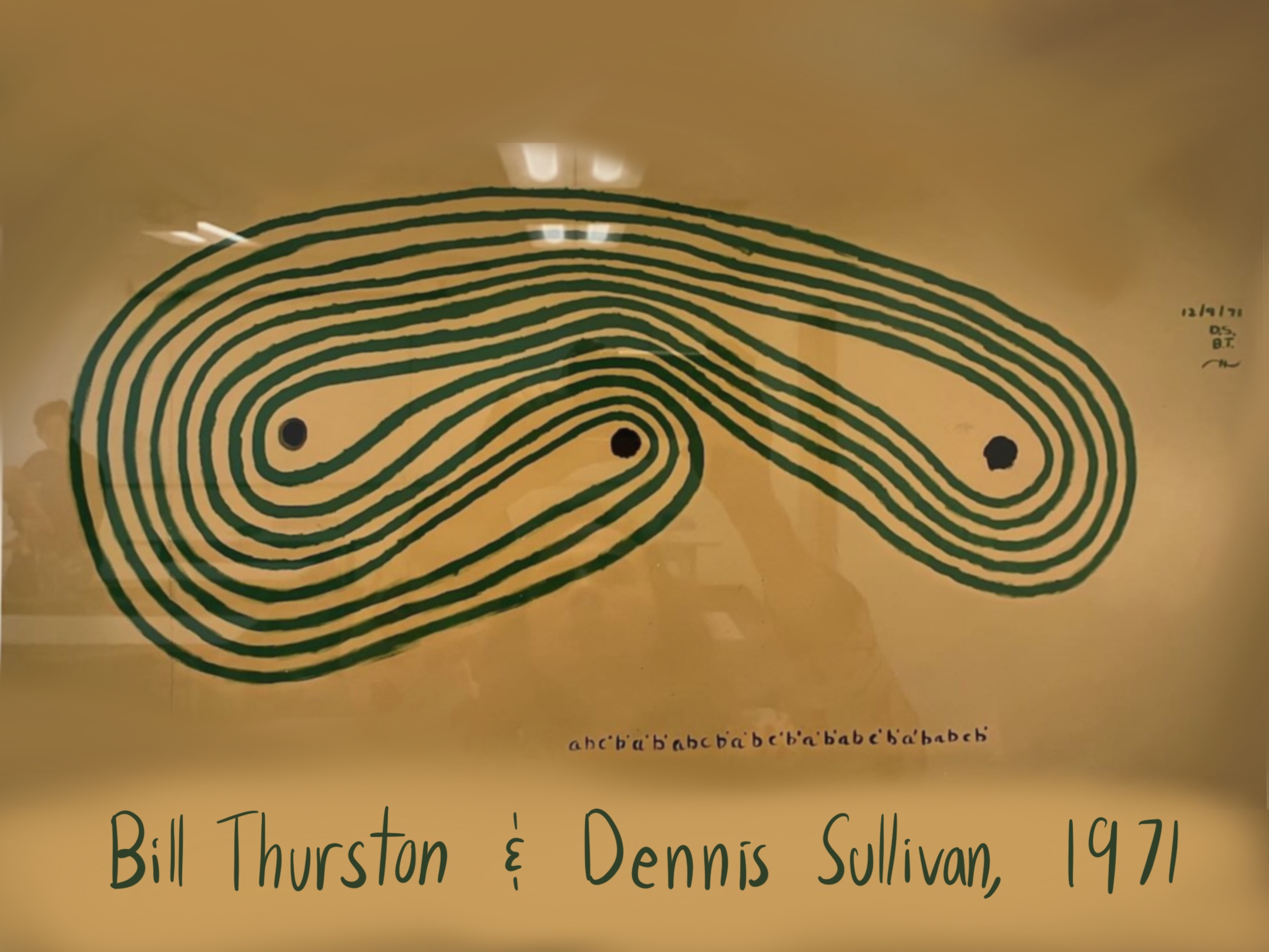
Mural from Evans hall
This is a picture of a single simple closed curve in a thrice punctured plane. Thurston built this curve iteratively, starting with a curve enclosing just two of the holes and “braiding” the holes around one another.
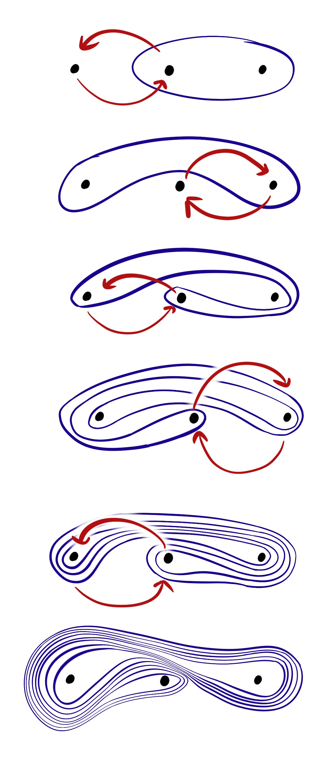
The curve gets stretched like taffy, folding over itself to form the curve of the mural. The mechanism is identical to Industrial candy makers. Thurston noticed that the curve quickly limits to sets of parallel strands which he called “laminations”. Sometimes the strands split apart into two groups, other times two groups merge. The mural ordaining the seventh floor of Evans hall showed Thurston’s nascent explorations of laminations, which would later blossom into his very influential theory of pesudoanosov maps. For Thurston’s description of the mural, see the last page of what is a train track.
Thurston encoded the structure of these laminations by collapsing the parallel strands into a single “train track”, a curve which can split or merge like the switches of a railway.
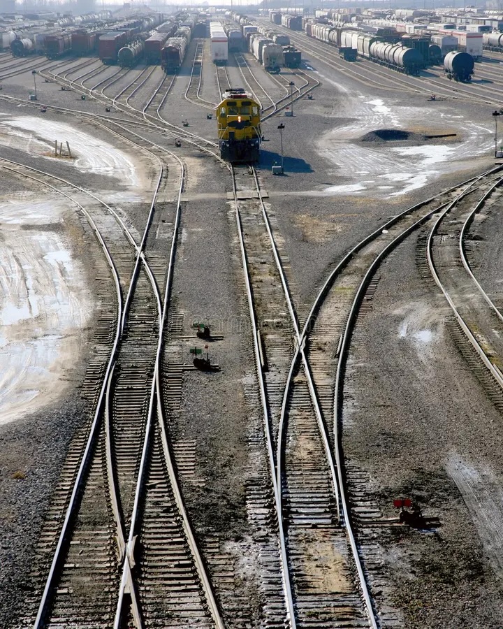
A real set of train tracks
Here’s the train track associated with Thurston’s mural. To build it, we lay “ties” across the lamination, then contract the ties to a central track.
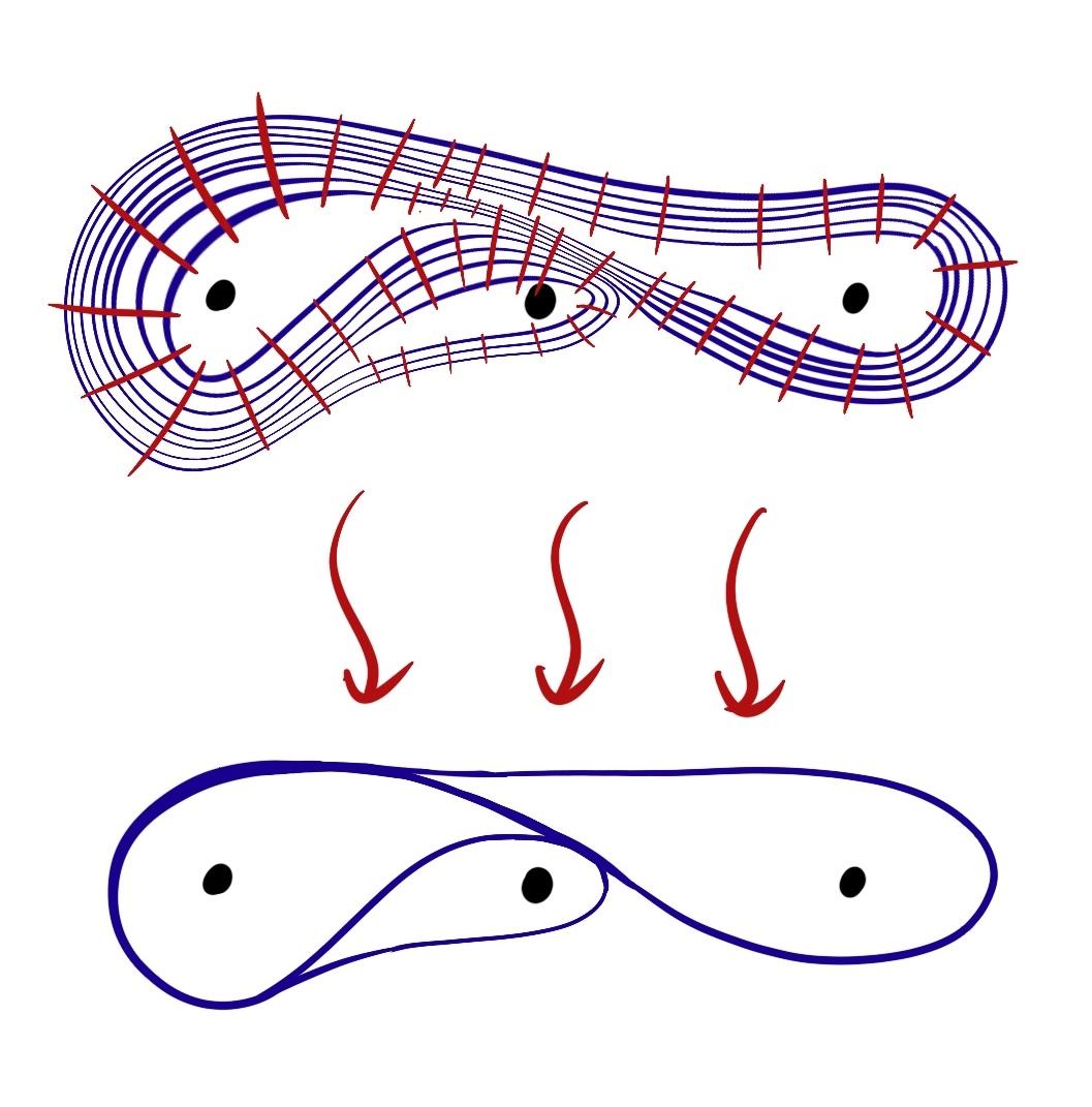
The first picture is a lamination. The second picture is the train track, formed by contracting parallel strands of the lamination.
The term “train track” was coined by Thurston alongside a handdrawn doodle of a little train puttering along these tracks, complete with a white puff of steam.
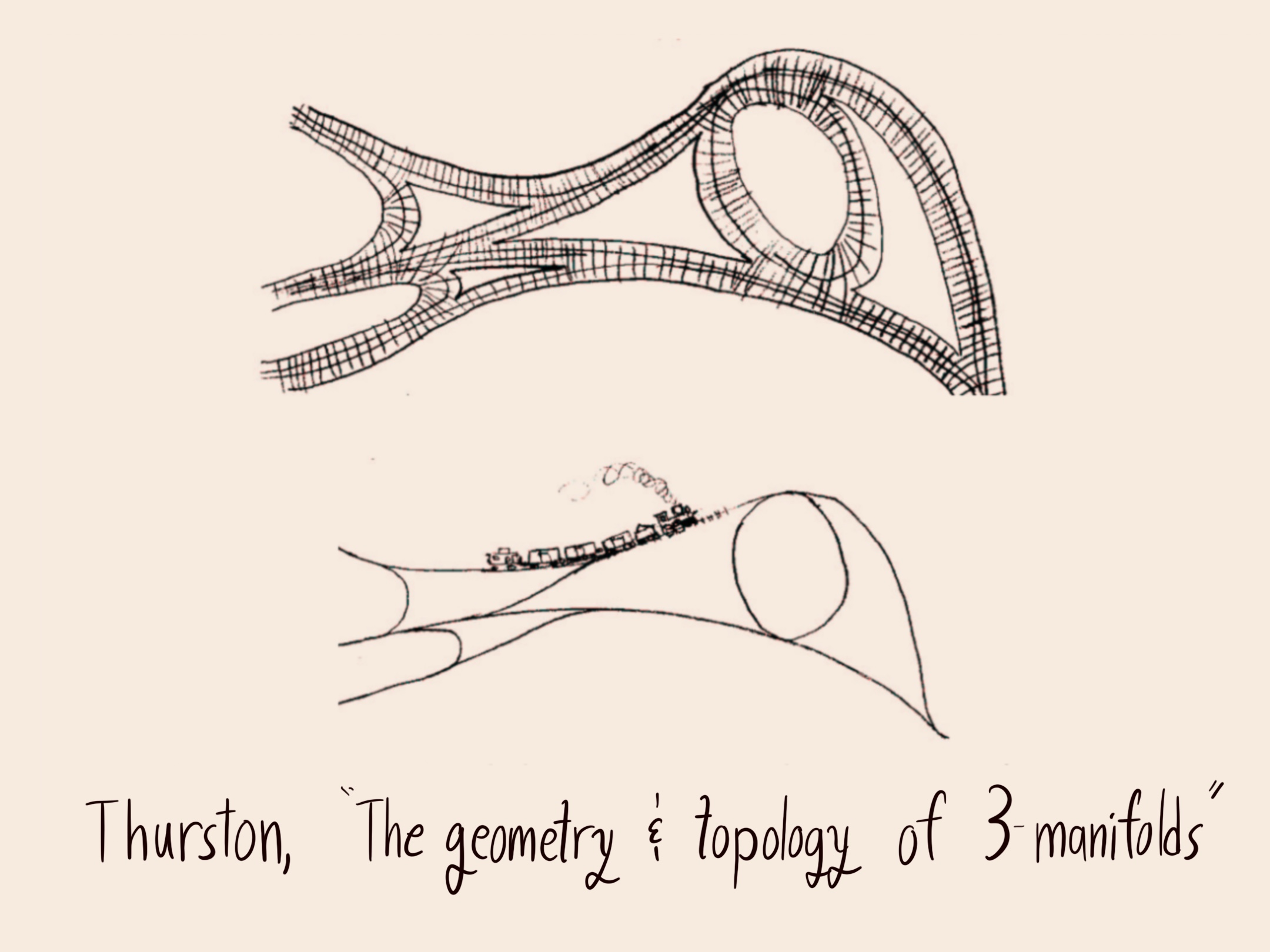
From The geometry and topology of three manifolds by Bill Thurston, chapter 8.9
How might we illustrate the idea of train tracks? Thurston made this task easy by naming it so evocatively, even giving us a sketch. This doodle inspired Conan Wu to draw this lovely piece:

By Conan Wu. For background, see her blog post.
This shows a train track winding around some higher-genus surface. This piece invites the viewer to “ride the train”, following the closed curve and bearing left or right at each switch. The very name, “train tracks” sets the scale. (Thurston famously believes that the best way to view a 3-manifold is by standing inside. Math is big for Thurston). Conan’s piece renders this beautifully, with the train encircling a planet plucked from “Le petit prince”. Here is her piece with an added person for scale.
This is a prime example of Big Math™. We know it’s big because the surface dwarfs the viewer, represented by our little friend. (By the way, the artist Conan Wu is living an very full life after her PhD, including a period as a concept artist and landscape painter at Disney.)
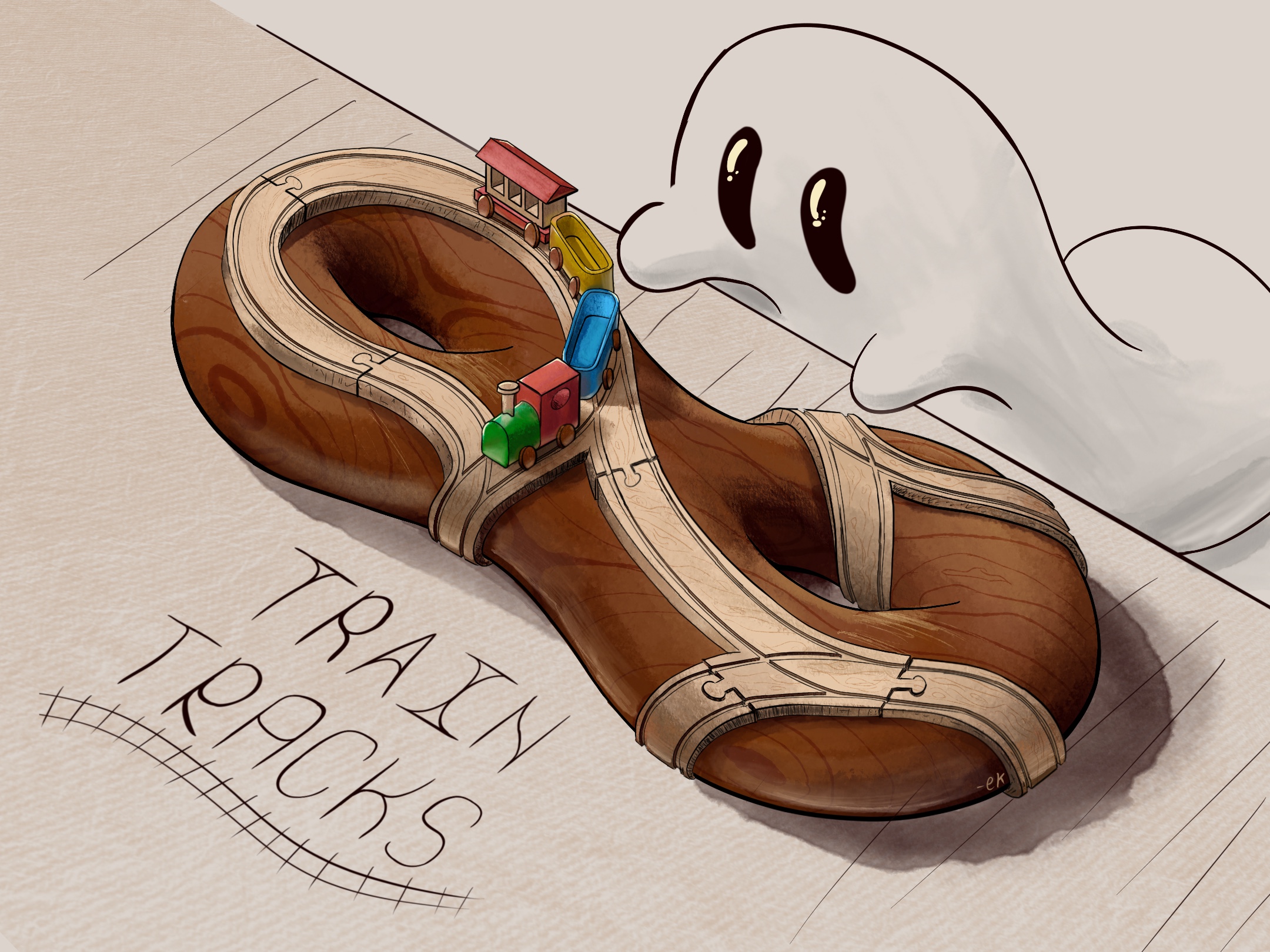
But what if we chose a different scale for our illustration? Here’s my take on the train track picture.
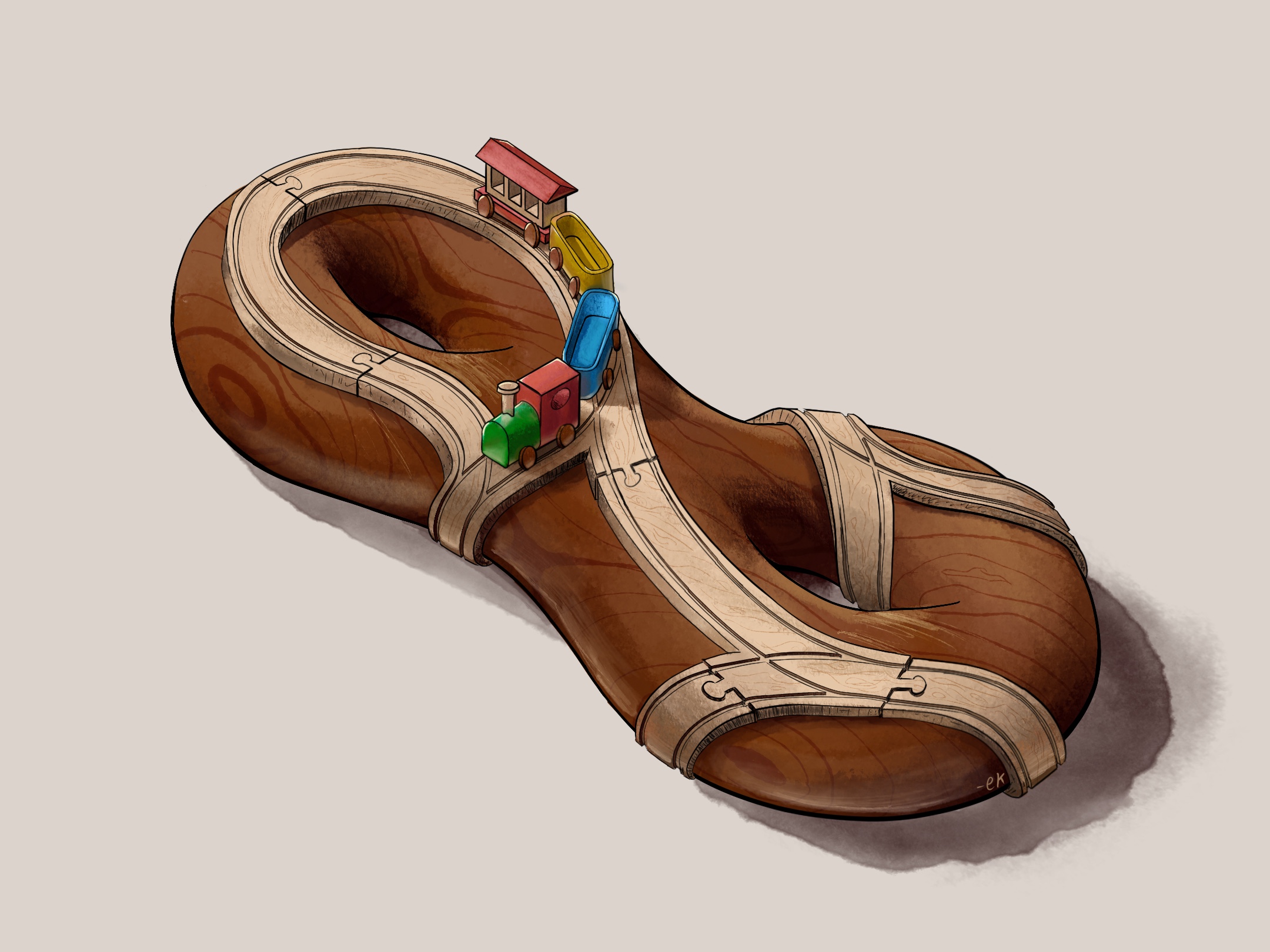
My picture of train tracks
I made the train a toy train, so the whole train track is something you can hold in your hand, or put under a Christmas tree. This is small math. This smaller scale begets different analogies. Instead of a old school locomotive to ride in, it’s a wooden train you push around. Instead of metal tracks, I used those wooden tracks that we played with as a kid. Where Conan’s planetary train track suggests emotions of awe or wonder, the toy one suggests fun and puzzles. Completely different emotional effects, for mathematically identical pictures.
Including the critter for scale, they are omnipotent. Instead of controlling the train as in Conan’s picture, the viewer is invited to piece together the tracks like legos. This emphasizes the combinatorial nature of train tracks. In contrast, in Conan’s picture the viewer is beholden to the shape of the planet and its tracks, Conan’s train revels in geometry.
Which scale should we pick? Is math big or small? I have two conflicting axioms about myself:
- I like small things
- I am a small
These are in conflict, for if I am small and surrounded by small things, then I am the same size as my things. Is math one of my little things, or something to immerse myself in? Let’s see what big math has to say for itself.
Big math in symplectic topology
For my day job, I study symplectic topology. I want to tell a story about one of the leaders of the field, Yasha Eliashberg. This will need some mathematical context, which I will try to keep light. Symplectic geometry is, succinctly, the study of symplectic manifolds. These are even dimensional manifolds with extra geometry called a symplectic structure. Here I represent the symplectic structure by the little critters climbing over the manifold.
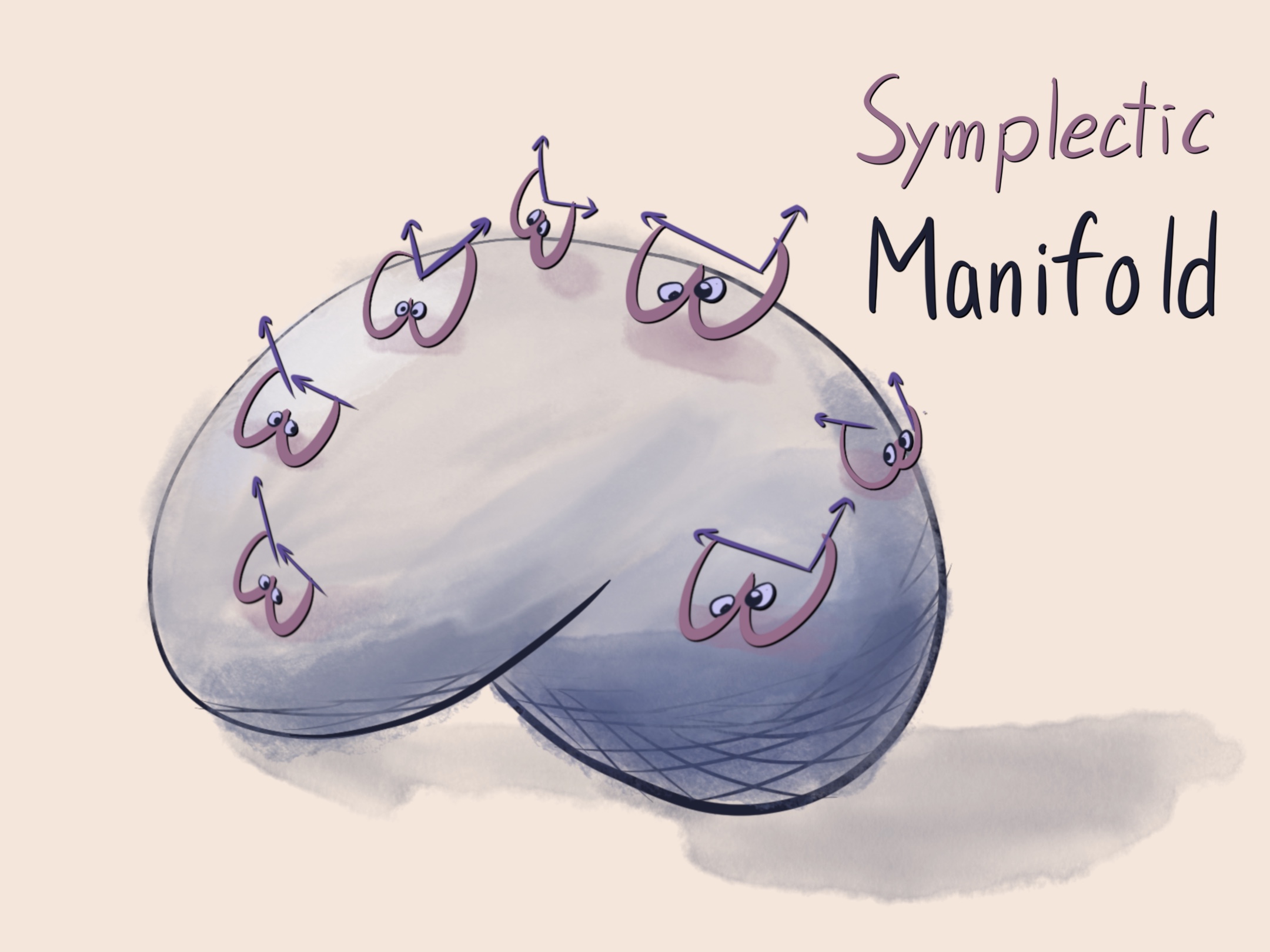
A symplectic manifold, crawling with symplectic forms.
The field kicked off in the 80s with the introduction of a tool called “pseudo-holomorphic curves”. These are two dimensional surface inside the symplectic manifold, stretched tight like a film of soap.
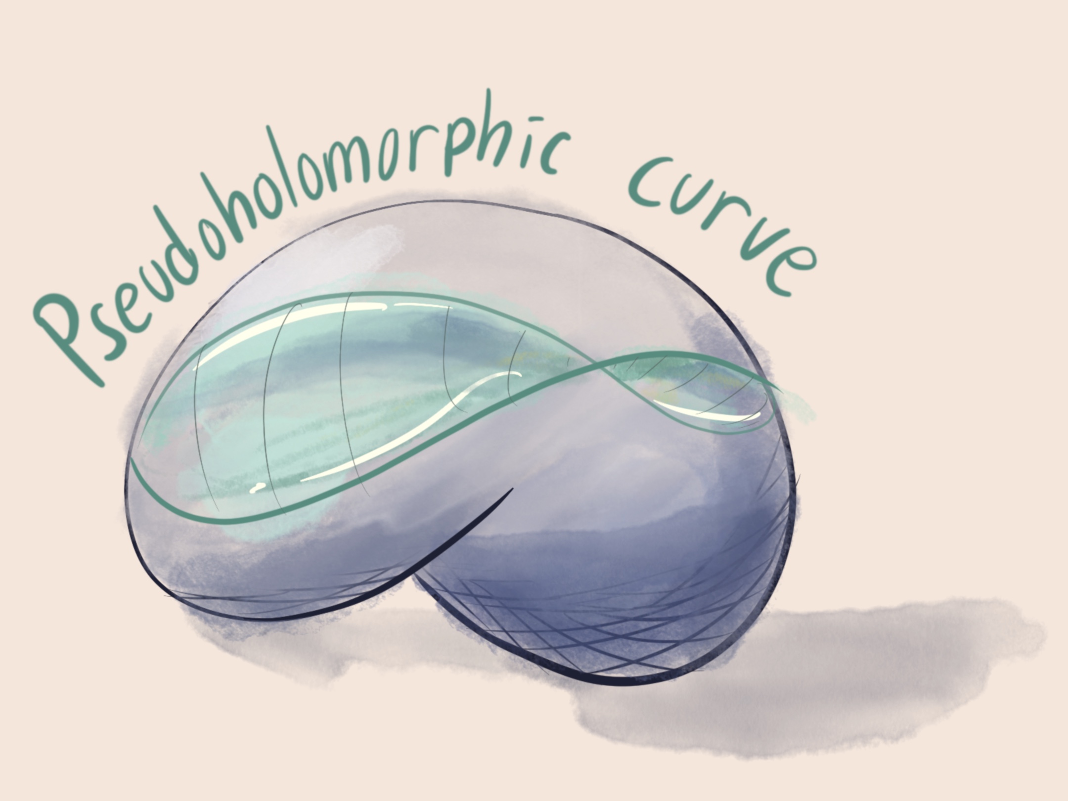
A pseudoholomorphic curve living inside a symplectic manifold
We understand symplectic manifolds by probing them with these pseudoholomorphic curves. A symplectic topologist makes their living by counting pseudoholomorphic curves, and using these counts to distinguish symplectic manifolds.
Yasha Eliashberg is one such symplectic topologist. Yasha is a 5’3, somewhat squirrelly yet animated fellow. In a conference held in his honor, “Yashafest”, one participant made an insightful quip:
“Yasha’s vision of mathematics is so great because he is very small”
Bourgeois reflects on this in his retrospective on contact homology
… Yasha imagines mathematical objects as being much larger than himself, so that he can visualize all their details and develop a good intuition. This is obvious for anyone who has had the chance to discuss mathematics with Yasha on a sidewalk terrace, where it would be typical for him to describe a huge pseudoholomorphic curve, coming from the other side of the street.
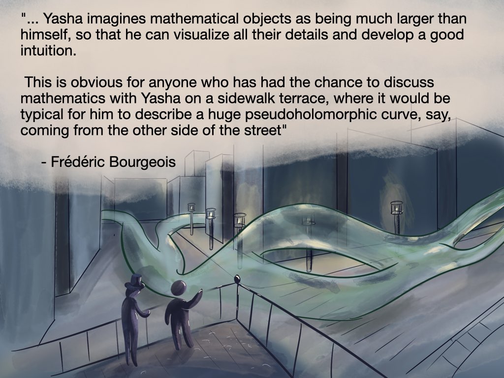
Yasha and Bourgeois, discussing pseudoholomorphic curves.
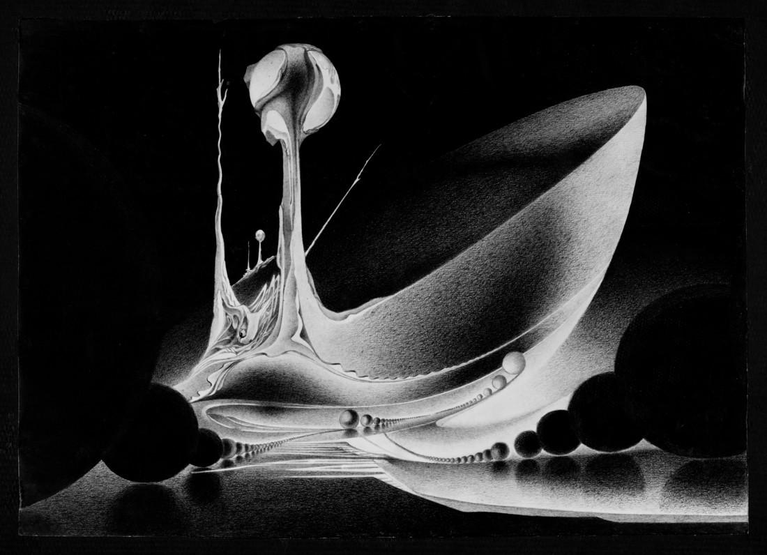
If we are to study the intricacies of pseudoholomorphic curves, we must walk among them. To Yasha, math is big. Yasha’s vision of math recalls the the imagery of fellow topologist and illustrator, Anatolii Fomenko. Here is how Fomenko conceptualizes a symmetric space. Fomenko’s math is monumental, equal parts awe-inspiring and imposing. Every detail dwarfs the viewer, demanding not to be ignored. You cannot have an ego exploring Fomenko’s world. Math is big, because you are small.
Yasha’s small perspective has quantifiably changed the imagery of the field. Let me explain one of Yasha’s major contributions, contact homology. Our goal is to count pseudolomorphic curves inside of symplectic manifolds. What if we take a symplectic manifold, and stretch it out like taffy? The resulting manifold has three parts: A left half, a right half, and a long neck connecting the two.
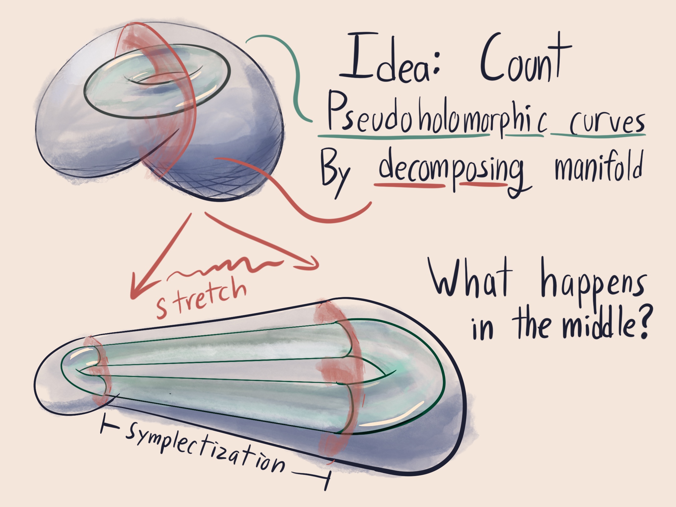
The idea which spawned symplectic field theory and contact homology
The pseudoholomorphic curve splits into the contributions from the three parts, the left and right, and the curve stitching the two halves together. Eliashberg, Hofer, and Givental thought to count curve by stretching apart the manifold, and understanding how curves behave in the long necks.
This neck is called a “symplectization”. You’ll notice I drew it as a cone. Indeed, in one direction the volume of a slice of the symplectization becomes very small, while in the other the volume is very large. I drew this below by making the symplectic critters smaller on the small side. This directionality is reflected in the possible pseudoholomorphic curves which probe the symplectization. we are allowed caps in the small direction, but not the large direction.
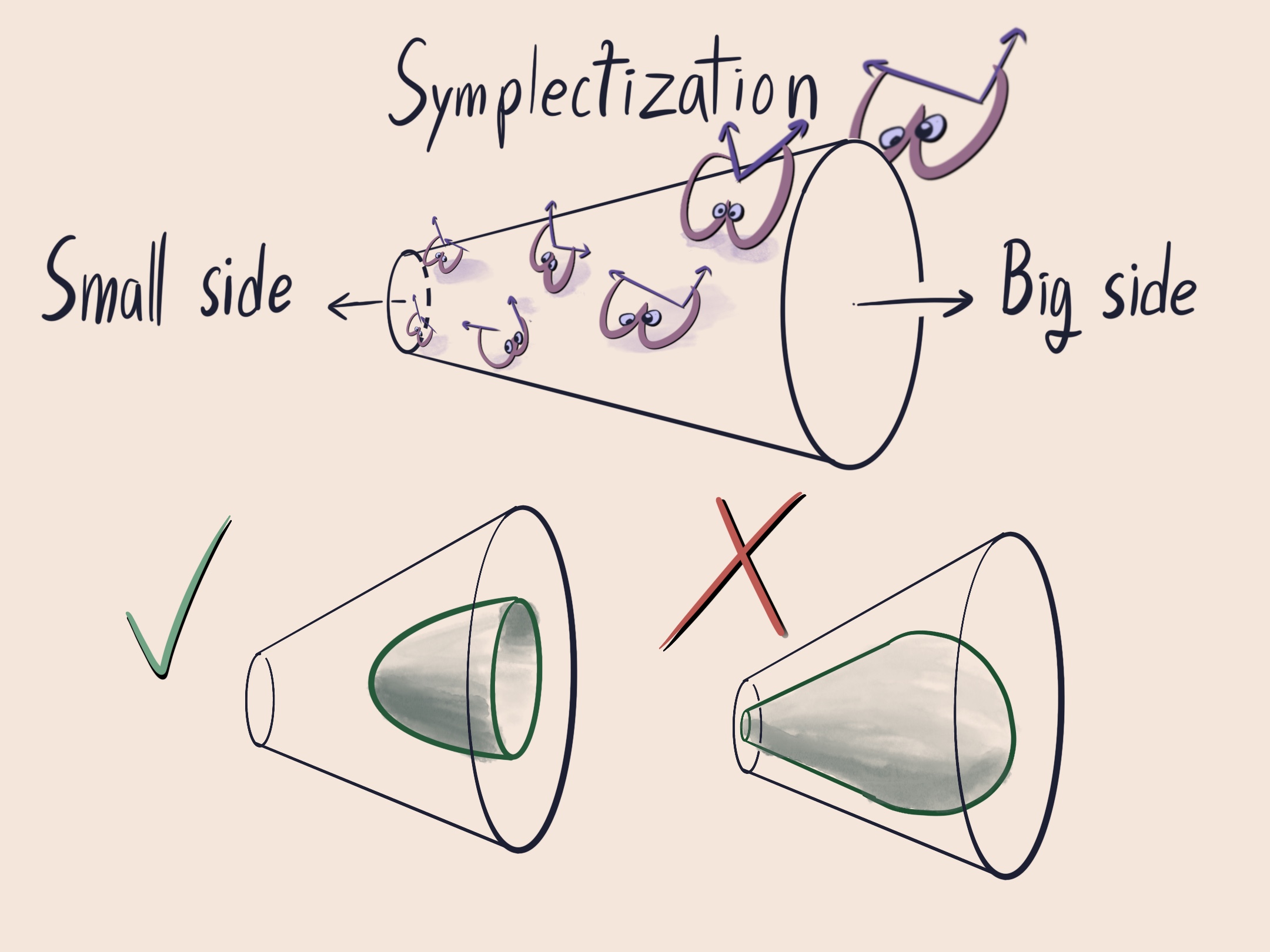
In symplectization, one direction is larger than the other.
Eliashberg figured out a way to extract an invariant from a symplectization, called contact homology. It requires counting pseudoholomorphic curves with one end in the large direction, but many ends in the small direction. The interesting mathematics happens on the small end. We can only see what the pseudoholomorphic curves are doing if if we zoom in to the small end.
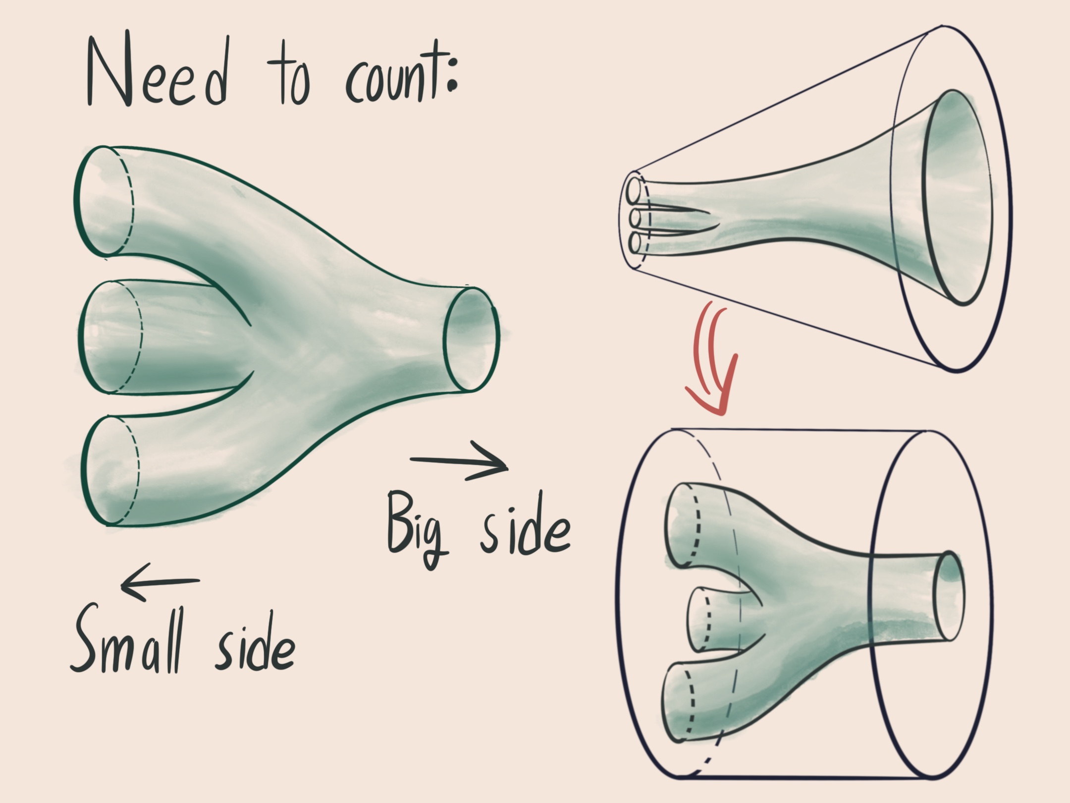
In contact homology, we count pseudoholomorphic curves with many ends in the small side of the symplectization. This suggests we draw symplectizations as cylinders.
This new point of view changed our diagrammatic for symplectization, for purely logistic reasons. With a conical drawing, we can’t draw what happens at the narrow end, because there isn’t enough room. Nowadays, people draw the symplectization as a cylinder. This confused me while learning, because the cylindrical drawing loses the directionality. Why should caps be allowed in one direction and not another? Which direction is which? In exchange, we can reason about the pseudoholomorphic curves relevant to geometry. Bourgeois muses that the discovery of contact homology took so long because we were still drawing symplectizations as cones. Math is big so that it can hold other math.
The cylinder is practical for the working mathematician. Contact homology endows curve counts with an algebraic structure, resulting from stacking multiple curves end-to-end. The cylindrical diagram is modular, with the small ends and big ends drawn at the same scale. Like the branching roots of a great tree, we can build multilayered pseudoholomorphic curves by drawing the diagrams one after another. Yasha and collaborators named these multilayered curves Pseudoholomorphic buildings. Something to walk around in. Yasha’s small perspective resonates throughout the field of symplectic topology.
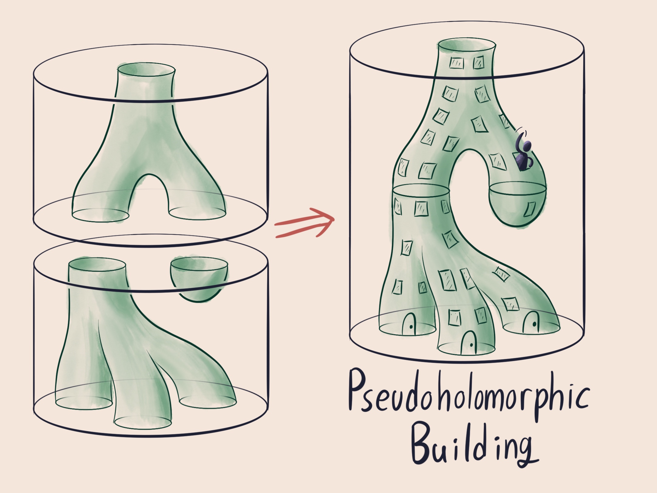
A "pseudoholomorphic building" is built by stacking pseudoholomorphic curves in symplectizations
Big math or small math?
Let’s review the benefits of big math exemplified by Yasha’s perspective on pseudoholomorphic curves.
- Imagining math as large lets you walk around inside it, and appreciate all its nooks and crannies. This perspective let yasha understand the intricacies of pseudolomorphic curves in the small side of the symplectization.
- Drawing something big lets you draw things inside it. This is why we now draw symplectizations as cylinders, so we can diagrammatically represent the relevant pseudoholomorphic curves
- The benefits of small math shine through in contrast
- Imagining math as small lets you manipulate it, grab it with your hands and rearrange things. This was the effect of wooden toy train tracks from earlier.
- Drawing something small lets you draw things outside of it. This lets us represent multiple objects and their relations with one another.
We see small math in the names of some math concepts. From combinatorics, there are domino tilings, which evokes toy dominos placed end-to-end on a table. the picture begs us to play with the math.
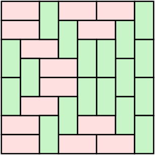
A domino tiling
From topology, you build larger manifolds by sewing together small manifolds. Multiple objects, attached together into a larger whole. If we want to change a single manifold, we can preform “surgery” cutting out a small part and sewing it back in a different way. Both these are operations on a manifold, so we must envision the objects as small if we are to control them.
Sewing manifolds. From my mathscape
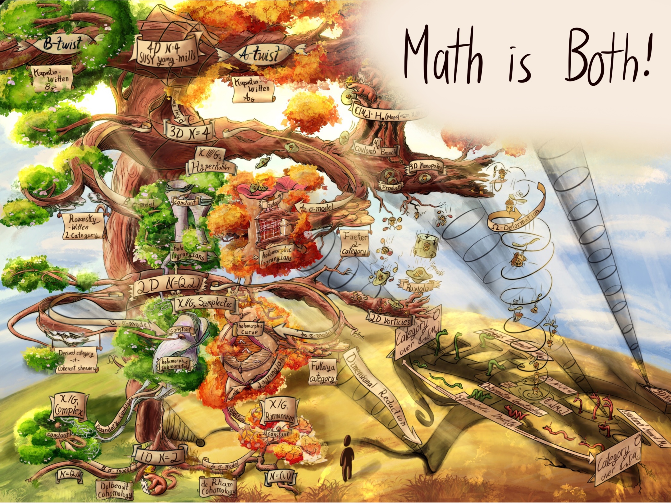
So which scale wins? Is math big or small? Well, both! Of course its both! How could it not be. Math is such an expansive field that it must be huge, but that doesn’t mean individual mathematical objects cant be small. Small things, living in a large landscape. Looking back at my own work, I’ve often used this separation of scale. Take this piece of mine, illustrating the interrelationships between various quantum field theories. The field theories are organized into a great tree, dwarfing the viewer (see our friend). Yet, the mathematical critters inhabiting each field theory are drawn as squirrels and acorns. The objects themselves are small in a big world.
Now we must place the line between big and small, and decide the viewers scale. Once again, we look to topologists for inspiration.
Geography and botany
A primary goal of mathematics is to classify mathematical objects. As our example for this section, we’re interested in closed curves in the 2 dimensional euclidean plane. It can be hard to tell whether two mathematical objects are the same, so the mathematician builds invariants, things we measure about objects to distinguish them. For curves in the plane, the two natural measurements are perimeter or area. If the perimeter or area of two curves differ, then the curves are certainly not the same.
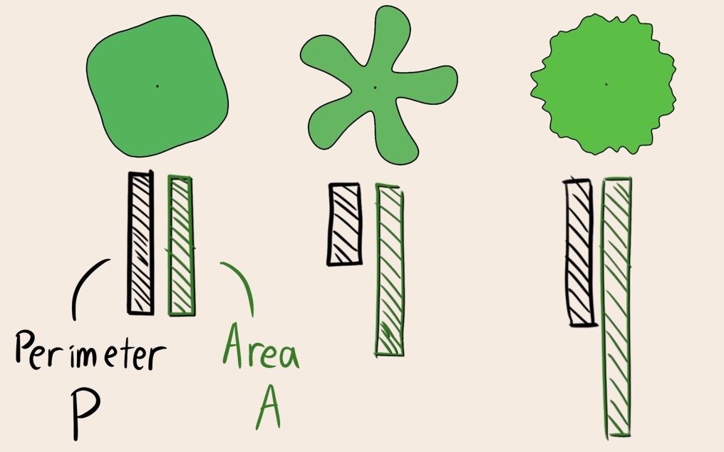
Perimeter and area of curves in the plane.
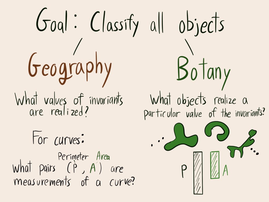
With a set invariants in hand, we can cut down the full classification problem into two subproblems, called Geography and Botany.
- Geography asks what possible invariants can be realized. In our example, which pairs of perimeter and area are realized by a closed curve?
- Botany asks to classify the objects realizing given values for the invariants. In our example, what are the curves with a specific perimeter and area?
Geography and botany
The names are certainly evocative, but it’s hard to see what they’re evoking without the picture. Take a closed curves, and measure their area $A$ and perimeter $P$. Then, plot the curve on $\RR^2$ centered at the point $(P,A)$. Here’s a few curves:
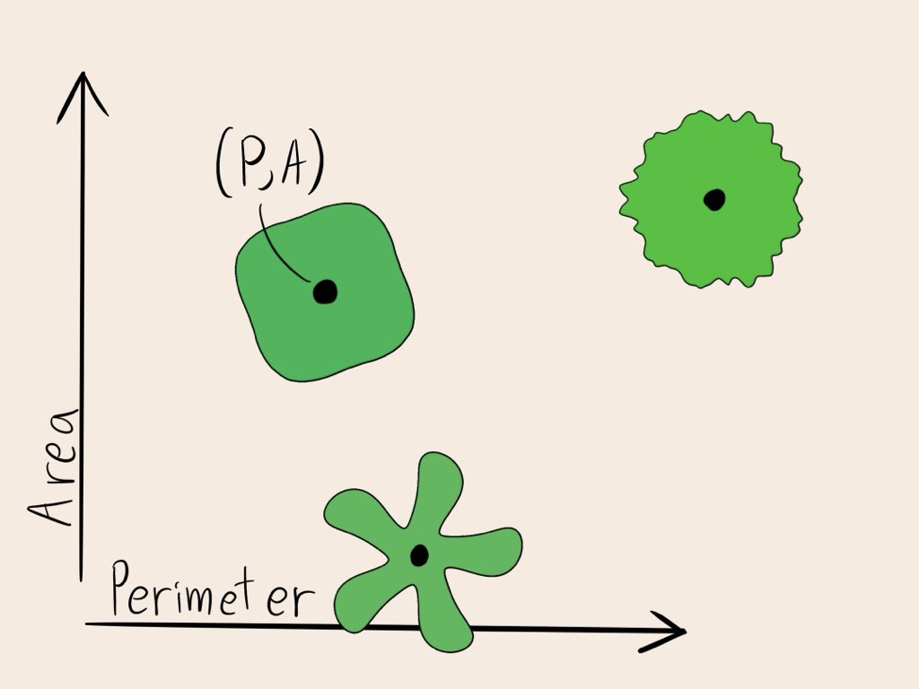
Plotting curves on perimeter-area parameter space
Here’s many curves
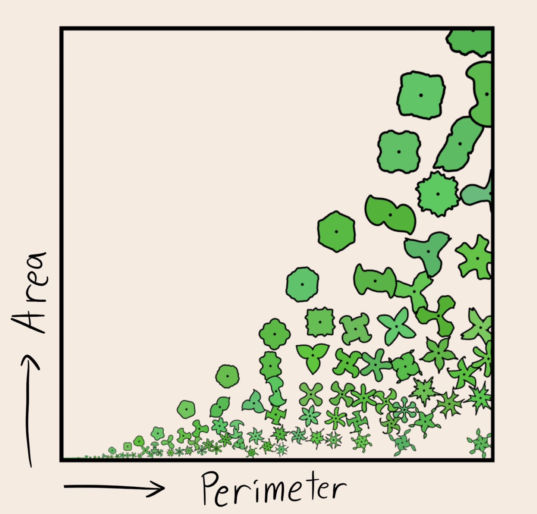
Let me take some creative liberty and shade the background:

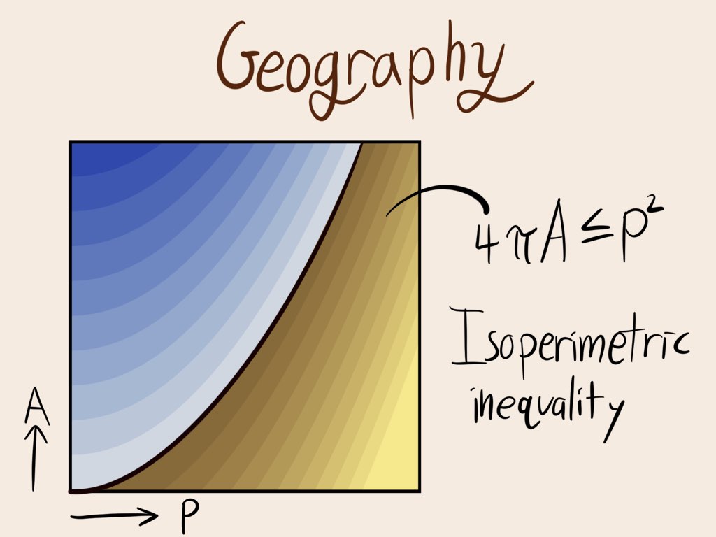
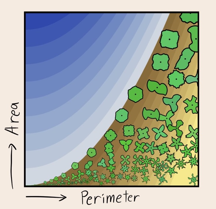
The isoperimetric island
Welcome to the isoperimetric island. This island is populated by flowers, each shaped like some closed curve. The $x$-coordinate of each flower is its perimeter, and the flower’s $y$-coordinate is its area.
First, notice the shoreline of the island. There are no flowers above a parabola shape. If we measure the parabola, we find that every flower satisfies the equation \(4 \pi A \leq L^2\)In words, a curve of fixed length can only ever enclose so much area. We’ve discovered the isoperimetric inequality! This solves the geography problem for area and perimeter.
Next, look at the flowers growing exactly on the coast. Each of them is a circle. Indeed, the circle is the unique shape maximizing enclosed area for a given perimeter. This solves the botany problem on the shoreline, where $4 \pi A = L^2$.
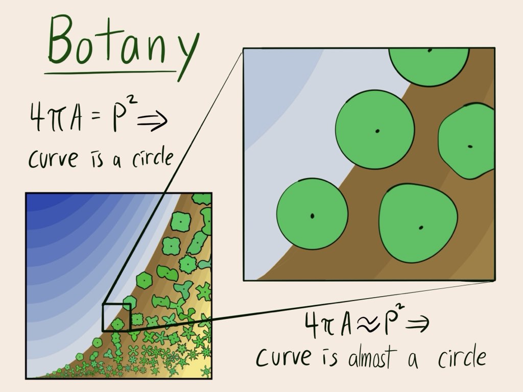
Moving inland, the flowers get more interesting. They develop crenelations, which become more and more pronounced the farther from the shoreline you get. We are observing the stability of the isoperimetric inequality. Any curve with $4 \pi A \approx L^2$ must be close to a circle. This characterizes the shape of flowers near the isoperimetric coast, tackling the botany problem near the coastline.
The “isoperimetric island” illustrates the analogy behind geography and botany. We envision math as an island, with mathematical objects as plants populating the island. Mathematicians, exploring the island, first act as geographers and map out the coast of the island, understanding the range of possibilities of the mathematical flora. As a geographer, math is big. Next, the botanists sit in place with a magnifying glass, classifying all the critters in that part of the island. As a botanist, math is small.
I find geography and botany a beautifully evocative analog which gives a precise scale. At the smallest scale are individual mathematical objects, plants under the preview of the botanist. Then is the mathematician, the viewer of the illustration. The largest scale is the collection of mathematical objects, an island to be mapped by a geographer. The viewer’s scale is right between the part and the whole.
This analogy is similar to Dyson’s delineation of mathematicians into Birds and frogs. It seems that every generation has a new dichotomy of mathematicians. I was told that Poincare divided mathematicians into poets and craftsmen (though I can’t seem to find a quote). I personally find that sorting people into boxes to be limiting, and unwelcome if someone else is sorting you. There is an implied value judgement praising the birds and the poets of math. But, Birds and frogs do both geography and botany. These are mathematically precise questions, modes of thinking that every mathematician must inhabit. The island analogy focuses on action rather than essence.
Using geography and botany
The geography and botany problems originate from topology. Almost all questions in topology are in service of the motivating question
Founding question of topology: Classify all manifolds.
The topologists primary tool are invariants. An invariant assigns a number to each manifold. If two manifolds are equivalent, every one of their invariants agree. Unless we’re very lucky, two manifolds with the same value for a certain invariant do not necessarily agree. Using a set of invariants, we split the classification problem into two smaller problems:
The geography problem: What values of invariants are realized by manifolds?
The botany problem: Classify the manifolds with given invariants
We’re classifying our manifolds by sorting them into bins according to invariant (geography), then understanding what fits in each bin (botany). If we fully understand both problems, we have classified all manifolds.
Complex curves
Let me give an example. A Riemann surfaces is a two dimensional manifolds with complex structure.
Goal: Classify Riemann surfaces
We consider two Riemann surfaces equivalent if they have the same topology and complex structure. Our topological invariant will be the genus, the number of holes in the surface. We can realize Riemann surface with every genus $\geq 0$, so we’ve solved the geography problem.
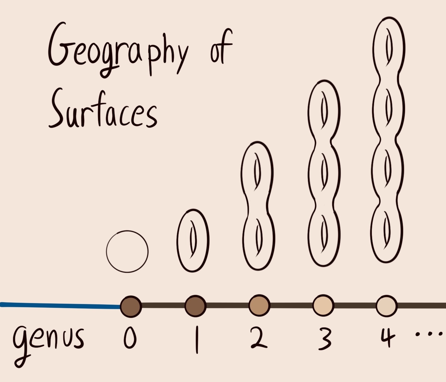
Geography problem on surfaces. A surface is classified by its genus, which can take any whole number value greater than or equal to zero.
Topologically, a surface is determined by its genus. The botany problem is trivial, because there is a single manifold with the given invariants. a single flower at any location of the island. But we are interested in the complex structure, making botany much more interesting. There are differently shaped nonequivalent Riemann surfaces with the same number of holes. Let’s analyze case by case.
- Genus zero: There is a unique Riemann surface. This solves the botany problem here. On the coast of the one-dimensional island, there is a unique flower, and it is $\mathbb{CP}^1$.
- Genus one: There is a two real parameter family of nonequivalent genus one surfaces. Over this part of the island, the flowers are tori with different widths and thicknesses. The botany problem asks to understand the space of such surfaces, which is called the moduli space of elliptic curves. We understand this fully.
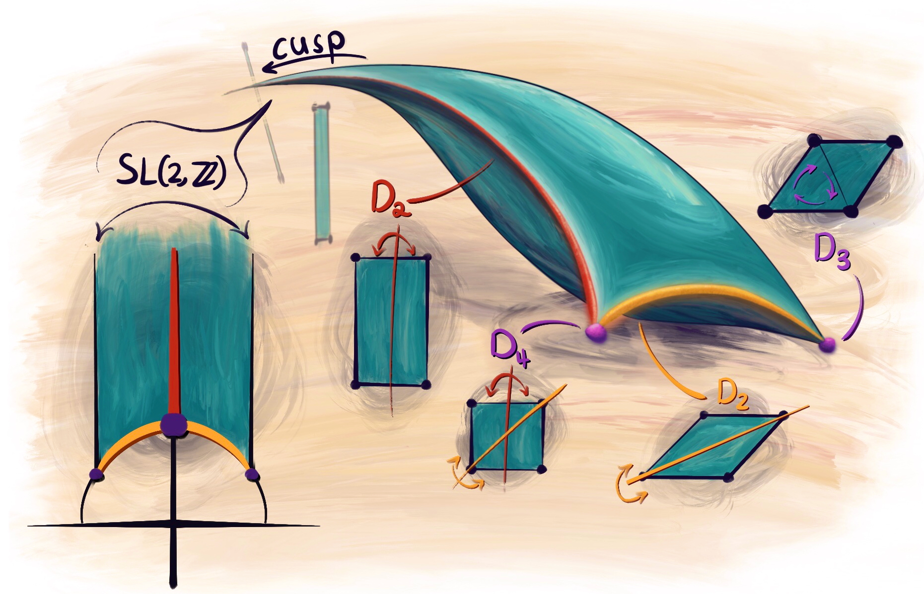
Moduli space of elliptic curves, from my paper
- For higher genus $g\geq 2$, the botany problem is much harder. The space of such curves forms a $6g-6$ dimensional space, the Riemann moduli space. These are some of the most studied spaces in mathematics, ever since they were introduced by Riemann in the 1850s, and are still studied to this day. The botany problem gets more and more complicated as you move inland, the biodiversity of the flowers increasing with the number of holes.
Complex surfaces
Riemann surfaces have a geography and interesting botany. Geography becomes more interesting one dimension up. A complex surface is a manifold with 2 complex dimensions, or 4 real dimensions.
Goal: Classify Complex surfaces
Once again, we need some good invariants. The natural choices are a pair of numbers called the Chern numbers, $c_1^2$ and $c_2$. Here is the geography of complex surfaces with respect to these invariants.
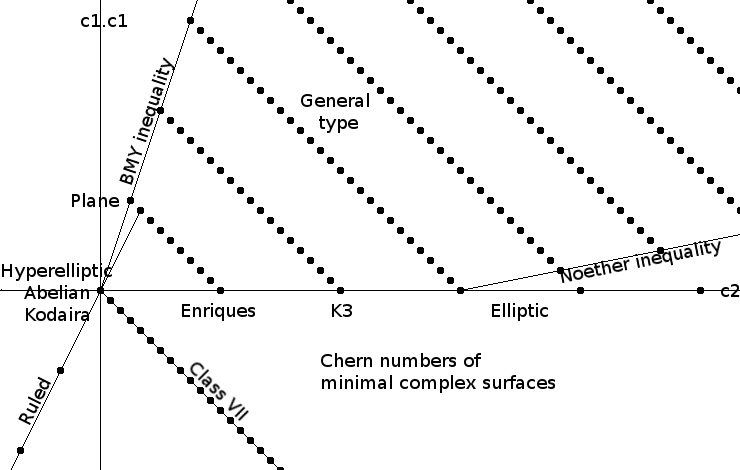
Geography of complex surfaces, from the Enriques–Kodaira classification
What a funky island! Let’s talk about the geography and botany together. We have the main bulk of the island, and a bunch of little jettes shooting off. Let’s just zoom in one one. In the bottom left, we have the ruled surfaces. We understand the botany for this part of the geography. Every surface over here is a bundle of spheres, living over a complex curve. We also have explicit descriptions for the class 7 jetty, and the “elliptic” line with $c_1^2 = 0$. the point $(0,0)$ is inhabited by several different species. The point $(0,2)$ carries $K3$ surfaces, critters which are all topologically identical, but have different complex structures. A K3 surface is defined by 19 complex parameters. Such rich botany, at a single point of the island!
And then there’s the main island, the overgrowth of “general type” surfaces. This is a jungle. We have no systematic classification of these surfaces, so their botany remains unsolved. This picture illustrates the classification of complex surfaces, which is the culmination of 19th and early 20th century algebraic geometry. It also visualizes the parts left uncharted, showing the boundary of our knowledge. Geography and botany organize the field.
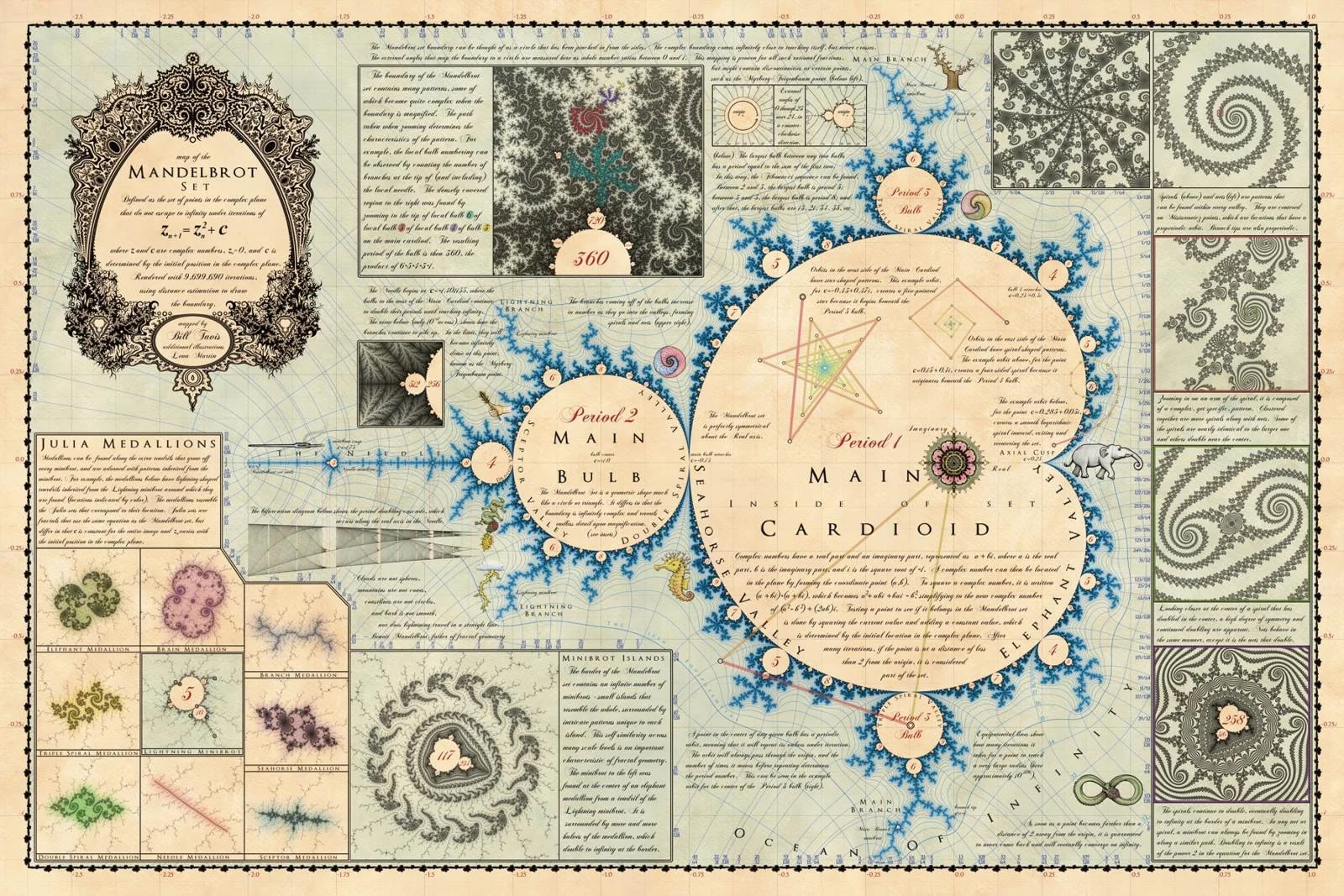
Mandelbrot sets
The Mandelbrot set is geography. Recall that a point $c\in \CC$ is in the Mandelbrot set if 0 diverges under repeated applications of the map $z \mapsto z^2+c$. We can think of the Mandelbrot set as a map of Julia sets. Under geography and botany, we should imagine the Julia sets sitting like flowers over each point in the Mandelbrot set. The Julia sets are small, the Mandelbrot set is big. This inspired artist Bill Tavis to make my favorite ever math poster, and render the Mandelbrot set like a vintage map.
The isoperimetric island
By Bill Tavis. Go Buy it here , it's a beautiful poster
Conclusion
Geography and botany are flexible analogies. Math is full of geography problems if you’re looking for them. Each of these problems can be rendered as an island to be explored by the viewer. Even if we change the coat of paint, geography and botany guides the scale. I’ve found them to useful for conceptualizing my own work, and to help answer my everpresent question: Is math big or small?
If you read this far, I imagine you think about math with analogies and pictures. I want you to reflect on the scale of those visualizations, and how that interacts with the underlying mathematics. If you think of something as small, try to make it big. If your math is already big, what would it look like if it were small? Which works best for you?
Gallery


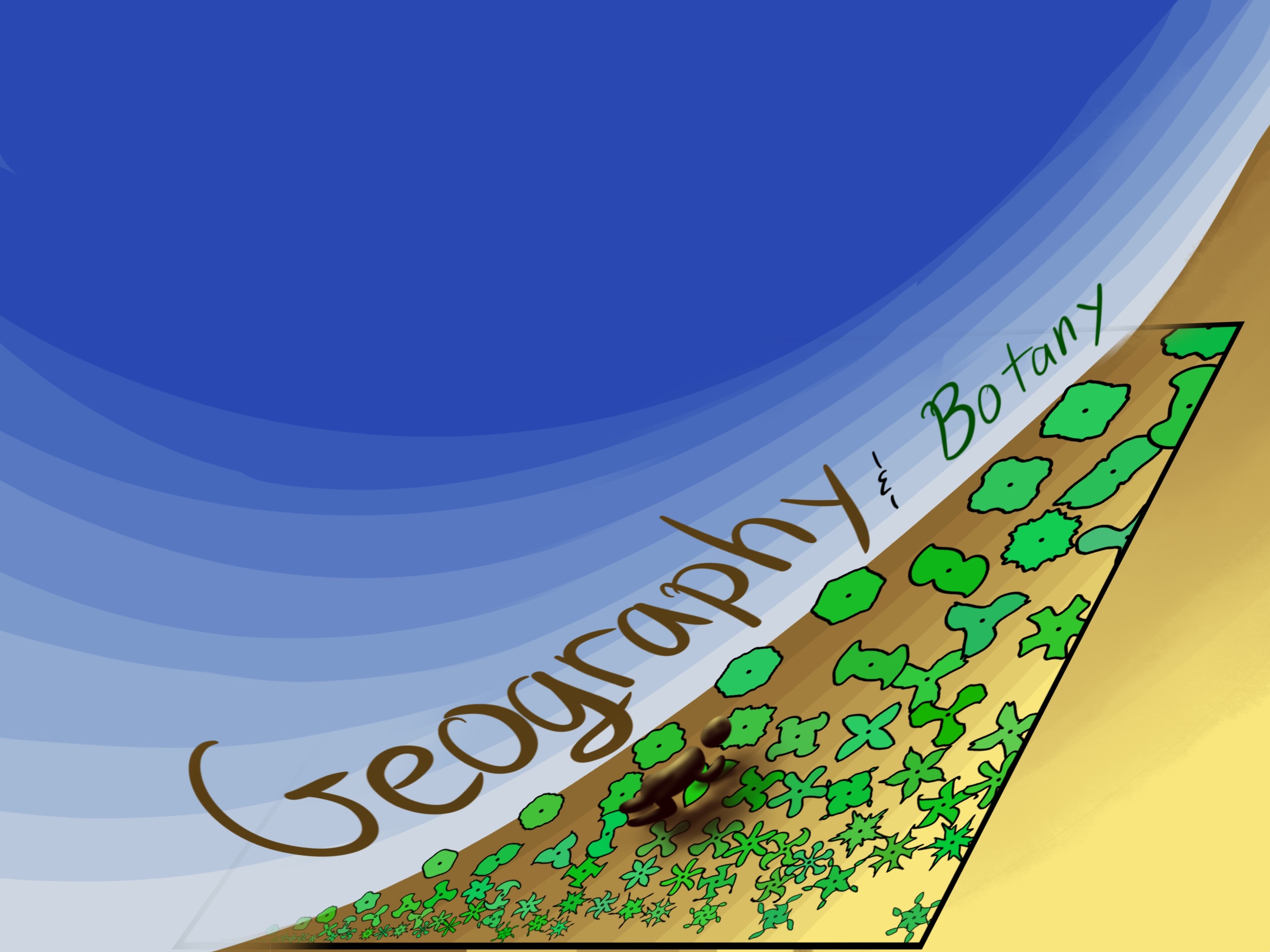
Is math big or small?
Title page for my talk. To make something seem big or small, you need a point of reference. I set the scale on this slide using the critters. You can read the talk on this very page