Illustrating the AI proof of the Mahler conjecture

Oct 2026

research expository art blog

Summary:

This week, OpenAI posted a proof of the Mahler conjecture, among about 400 other problems. One of the proofs goes through symplectic geometry, constructing a symplectic embedding of a ball of the right volume into $K \times K^\circ$. In this post I illustrate the techniques of this proof, and draw the image of this symplectic ball.

[!epigraph] Srinivasa Ramanujan (apocryphal (I made it up)) The machines may prove my theorems, but they will never prove my spirit!

Slop day has arrived, and we must reckon with the aftermath¹. Of the 373 solutions released by OpenAI this Tuesday, I’m most interested in #087, a proof of the Mahler conjecture. Like many other mathematicians, I’ve been scooped :(. The AI proof is a clever construction applying a technique I haven’t published yet. My result wasn’t groundbreaking. It was a cute, self-contained thing with a simple proof (imo the best kind). I thought it could be quite useful (apparently so!) but I haven’t finished my application. The Mahler conjecture was on my list of things to try eventually. Ah well. Nothing to do but plant a flag in one of the 400 plots of the wasteland.

I’m most interested in the symplectic aspect of the Mahler conjecture. For an $n$-dimensional symmetric convex body $K$ and its polar $K^\circ$, AI constructs a symplectic embedding of a ball of radius $2/\sqrt{\pi}$ into $K\times K^\circ$. As a corollary, the volume of the product is greater than the volume of the ball, $\Vol(K \times K^\circ) \geq \frac{4^n}{n!}$. This settles the longstanding Mahler conjecture (along with two other AI papers, characterizing equality and proving the non-symmetric version). This problem is one of the few with a summarized chain of thought, which is honestly kinda insulting. In the 45-page document, the discussion of the symmetric case occupies a grand total of one paragraph.

In this post, I’ll first explain the words in the paragraph above, and why we care. This will be accessible to a broad mathematical audience. In the second part, I’ll motivate, illustrate, and sketch the proof from the AI paper, written for symplectic geometers.

Morals and motivation

I have two motivations for writing this post. Mathematically, I want to be a human for these ideas. I’ve been thinking about half of this (producing symplectic balls in holomorphic sub-manifolds) for the last three months. This AI result is a really cool application. If anyone wants to discuss other applications, I’m happy to chat :)

Second, I’m modeling the role of mathematical illustration in a world of AI, where proofs are cheaper than understanding. Rather than “digesting” the proof, I’m “illustrating” it, in the sense discussed in “On the importance of illustration for mathematical research”. AI coding has democratized the technical skills needed for interactive visualizations — I wrote all the programs in this article in a couple of days. Unaided, the machines produce visualizations that are correct and flashy, evident from all the vibe-explanations of math you see on Twitter. We must strive for a higher standard, for rigorous illustrations. When the process behind the illustration is born from the mathematics it illustrates, the creation and illustration of math merge into one. In this post, my main visualizations draws a four dimensional shapes via slicing. This slicing is both illustrative and mathematical, being the exact slicing used in the proof. The illustration is rigorous.

I spent a trimester in Paris with the math illustration community, trying to make notions like rigorous illustration precise (see what I made here). I believe that illustration has an important role to play in our new age of math, as argued in the article Mathematical Illustration: Proof, Intuition and AI. You too can make illustrations. All it takes is care.

AI disclosure

All text and hand-drawn figures in this document were made by me. I vibecoded all the applets with Claude Code, and had AI assist with website layout. I used Claude to help read the AI paper, and to mathematically and grammatically proofread this document.

Contents

• Background
  • The Mahler conjecture
  • Symplectic capacities and the Viterbo conjecture
• Proof
  • Symplectic monotonicity theorem
    • Proof of
    • Visualizing the symplectic balls
  • Constructing the holomorphic submanifold
    • Limiting with $L^\infty$ norms
    • A first guess at a holomorphic submanifold
    • Building $K\times K^\circ$ when $n=1$
    • The magic map $g$
    • The holomorphic submanifold construction
  • Visualizing the symplectic balls in $K\times K^\circ$

Background

The Mahler conjecture

Every math field comes with its very own duality. The originator is linear algebra, where a vector space $V$ is dual to the space of one-forms $V^\ast$. This manifests in Euclidean geometry as a duality between points and half-spaces. Each one-form $\alpha$ defines a half-space containing the origin, $H_\alpha = \lbrace v \in V \, \big \vert\, \alpha(v) \leq 1\rbrace$. In polyhedral geometry, a convex polyhedron can be described as either the convex hull of its vertices, or as the intersection of half-spaces corresponding to its facets. The vertex and facet descriptions are dual.

The fundamental duality in convex geometry is polar duality. For a convex body $K \subset V$ define the polar $K^\circ \subset V^\ast$ as the collection of half-spaces containing $K$. That is,

The convex body $K$ is thought of as a set of points, while its polar $K^\circ$ is a collection of hyperplanes. Identifying $V$ with $V^\ast$ using the Euclidean metric, we can compare pictures. Play around with these in 2D to get a feel. Try making $K$ long and skinny, and see what happens to $K^\circ$.

[!sketch] mahler conjecture/polar polygon A symmetric polygon $K$ and its polar $K^\circ$. The defining half-spaces of $K$ correspond to the vertices of $K^\circ$.

The polar operation behaves nicely.

• $K^\circ \subset V^\ast$ is convex. If $K$ is closed, symmetric and convex, then $K^{\circ\circ} = K$. The polar is an honest duality relation.
• $(\lambda K)^\circ = \frac{1}{\lambda}K^\circ$. Scaling up the body scales down its polar.

Exploiting the scaling property, we can build a scale-invariant quantity from $K$ and its polar. Let $\vert K\vert$ denote the volume of $K$. Define the Mahler volume as the product of volumes of $K$ and its polar:

The largest possible Mahler volume is achieved by a ball, $M(K) \leq M(B(1))$. The minimal Mahler volume was, until now, unknown.

[!conjecture] Mahler conjecture Suppose $K$ is symmetric, meaning $K = -K$. The minimal Mahler volume is achieved by a cube.

\[M(K) \geq M([-1,1]^n) = \frac{4^n}{n!}\]

We can think of Mahler volume as a measure of roundness. The (unique) highest roundness shape is a ball, the (non-unique) lowest roundness symmetric shape is a cube. For more details, history, and intuition, see Terry Tao’s blog. This problem has been kicking around for at least 100 years, and has inspired some beautiful bridges between convex geometry and several complex variables. It also ties closely with symplectic geometry.

Symplectic capacities and the Viterbo conjecture

Let us combine $K$ and $K^\circ$ into a single object, their Cartesian product $K \times K^\circ \subset V \times V^\ast$. We will be making a lot of pictures of this space, and now is a good time to set the visual language. We will always draw two dimensional bodies $K$, so $K\times K^\circ$ is a four dimensional shape. The two main ways to render a 4 dimensional object is through projection or slicing. Here’s the projection onto the screen, so you can look around.

[!sketch] mahler conjecture/polar product On the left, The product $K\times K^\circ$, projected from $V\times V^\ast$ to the screen. In the middle is the view selector. place the red selectors in the middle to long along the red dimension, and vice versa for the green selectors. On the right, a selector for the polygon $K$ and its dual $K^\circ$.

A lot going on, right? Slicing will be more understandable for us. For any shape $\Omega \subset V\times V^\ast$, denote the slice above a point $x\in V$ as $\Omega^x = \Omega \cap \lbrace x \rbrace \times V^\ast$. By stacking all the slices $\Omega^x$ next to each other, we reconstruct $\Omega$. When $V$ is two dimensional, we can draw $\Omega$! Let the screen represent $V$. For a representative array of points on $V$, draw a scaled down copy of $\Omega^x$. Lining these up next to one another, our eyes notice the changes in the slices for each $x$. Applying this technique to $\Omega = K \times K^\circ$ is not so exciting, since every slice is the polar $\Omega^x = K^\circ$. Later on, we will see the slices change with position.

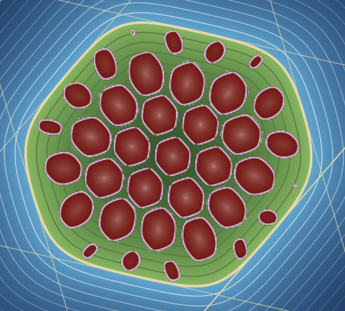
[!sketch|square] mahler conjecture/hexagonal grid/polar.html Visualization of $K\times K^\circ$. You are invited to think of $K$ as an island, and the small copies of $K^\circ$ as flowers populating the island. This visual metaphor is inspired by geography and botany.

Geometrically, the ambient space $V \times V^\ast$ is a cotangent bundle $T^\ast V$, which carries a natural symplectic structure (i.e nondegenerate 2 form). In coordinates, if $V$ has coordinates $q_i$ and $V^\ast$ has dual coordinates $p_i$, then $\omega_{std} = \sum \de q_i \wedge \de p_i$ is the symplectic form. This makes $K\times K^\circ$ into a symplectic domain, whose symplectic volume equals the Mahler volume. Motivated by the Mahler conjecture, is there a uniform lower bound for the symplectic size of $K\times K^\circ$?

We formalize the notion of symplectic size with a symplectic capacity. Consider a machine $c$ which takes a symplectic domain $(D,\omega)$ and outputs a real number $c(D,\omega)$ (we will often use $c(D)$ as shorthand when the symplectic structure is implicit). In order for $c$ to represent symplectic size, it must satisfy a few axioms. First, it must be symplectic.

1. Symplectic invariance: for any diffeomorphism $\psi:D \to D’$, we have $c(D’,\omega) = c(D,\psi^\ast\omega)$.

Second, it must be a “size”. For any good notion of size, if a domain $D$ fits inside of $D’$, then the size of $D$ is less than or equal to that of $D’$. In the symplectic world, to fit is to symplectically embed. A map $\psi:(D,\omega) \hookrightarrow (D’,\omega’)$ is a symplectic embedding if it is an embedding satisfying $\psi^\ast \omega’ = \omega$. This motivates our second axiom.

2. Monotonicity: If there exists a symplectic embedding $\psi:D \hookrightarrow D’$, then $c(D) \leq c(D’)$

Anything satisfying $1$ and $2$ is a symplectic measure of size. For our sanity, we demand that the size scales linearly with the symplectic form.

3. Scaling: $c(D,\lambda \omega) = \lambda c(D,\omega)$.

A machine $c$ satisfying axioms $1-3$ is known as a symplectic capacity.

The quintessential capacity is the Gromov width $c_{Gr}$, which measures the largest ball that symplectically embeds inside the domain. To fix notation, we define some standard symplectic domains. Pick coordinates $q_i$ on $V$, and dual coordinates $p_i$ on $V^\ast$. Define the ball $B^n(A)$ and a cylinder $Z^n(A)$, which are symplectic domains endowed with the standard symplectic form

These are parametrized by their two dimensional cross-sectional area $A$. Define the Gromov width:

For example, Gromov’s non-squeezing theorem states that $c_{Gr}(Z^n(A))=A$, meaning a ball cannot symplectically embed into a cylinder with smaller cross-sectional area. You can’t squeeze a ball into a smaller tube.

A bold conjecture from 2000 posits that many measures of symplectic sizes agree on symmetric convex bodies. Say that a symplectic capacity is normalized if $c(B^n(A)) = c(Z^n(A))$. For example, the Gromov width is normalized.

[!conjecture] Strong Viterbo conjecture Let $c,c’$ be normalized symplectic capacities. Then for any symmetric convex body $\Omega \subset T^\ast V$, the capacities agree

\[c(\Omega) = c'(\Omega)\]

[AAKO]² showed that the Mahler conjecture is a corollary of the Viterbo conjecture. Specifically, they proved that the Hofer–Zehnder capacity $c_{HZ}$, another normalized capacity, satisfies $c_{HZ}(K \times K^\circ) = 4$. Viterbo’s conjecture implies

That is, there is a symplectic embedding of a ball of width $4$ into $K \times K^\circ$. Since symplectic maps preserve volume, this gives a lower bound on volume.

matching the lower bound conjectured by Mahler! This paper was fairly influential, and spurred renewed interest in Viterbo’s conjecture, which continues to be a driving problem in symplectic geometry (until the next AI drop…)

The result du jour realizes this story:

[!theorem] AI The Gromov width of $K \times K^\circ$ equals $4$.

This does not go through any sort of Viterbo conjecture, though it does imply the Viterbo conjecture for $K\times K^\circ$. Perhaps the techniques could be strengthened to the full Viterbo conjecture.

The AI proof explicitly constructs a symplectic embedding of a ball $B^n(4)$ into $K\times K^\circ$, supplying a lower bound $c_{Gr}(K\times K^\circ)\geq 4$. Combined with the upper bound $c_{Gr}(K \times K^\circ) \leq 4$ on the last page of [AAKO]², this gives the result. The AI seems very capable at creating crazy symplectic embeddings, evidenced by their construction of high dimensional ball packing.

Proof

I will present the proof as if it were written by a colleague, assuming it’s correct and outlining the ideas. I haven’t checked the line-by-line details (which is important, because this paper doesn’t come with a Lean proof). The proof has two parts. First, it embeds a symplectic ball in the intersection of a holomorphic submanifold with a ball. Second, it constructs a sequence of holomorphic submanifolds which, when intersected with a ball, is a subset of $K \times K^\circ$. Stated as theorems,

[!theorem] Symplectic monotonicity formula (section 2) Let $i: M\hookrightarrow \CC^N$ be a smooth holomorphic submanifold passing through the origin, endowed with the pullback of the standard symplectic form $\omega = i^\ast\omega_{std}$. Consider the intersection of $M$ with a ball of area $\pi \lambda$ centered at the origin, $M^{<\lambda} = M\cap B^N(\pi \lambda)$. The Gromov width of $M^{<\lambda}$ is bounded from below by that of the ball

\[c_{Gr}(M^{<\lambda},i^\ast\omega) \geq \pi \lambda.\]

If $M$ intersects zero with multiplicity $k$, then for a desingularizing symplectic form $\omega_0$,

\[c_{Gr}(M^{<\lambda},i^\ast\omega + \omega_0) \geq \pi k\lambda.\]

The first part of this theorem is going to be a central result in my upcoming paper, so I guess I got scooped. The rest of the proof is a clever construction of the holomorphic submanifold. A convex body $K$ is a limit of symmetric polyhedra (section 5), which are the intersection of symmetric strips. From now on, assume $K$ is the intersection of $N$ strips defined by vectors $b_i$, meaning

[!theorem] Holomorphic submanifold construction (section 4) Define $\ell_i(z) = \langle z,b_i\rangle$ to be the complexified linear functional determined by each strip. For a holomorphic function $g:\CC\to \CC$, define a holomorphic map $f_k:\CC^n \to \CC^N$ by

\[f_k(z) = (g(\ell_1(z))^k , \dots, g(\ell_N(z))^k)\]

and denote its image by $M_k = f_k(\CC^n)$. The intersection with the unit ball $(M_k^{< 1},f_k^\ast\omega_{std})$ is symplectomorphic to a domain in the symplectic vector space $(D_k,\omega_{std}) \subset \CC^n$. There exists a function $g$ such that as $k\to \infty$, the domain $D_k$ is a subset of $K \times \frac{\pi k}{4} K^\circ$.

Explicitly, $g$ is a conformal transform from a lens-shaped domain $L\subset \CC$ to the unit disc $\mathbb{D}$ such that the angular coordinate on $\del \mathbb{D}$ pulls back to the $x$-coordinate on $\del L$ (Constructed by Gross in the context of Brownian motion).

[!figure|600] Key conformal map Drawing of the lens domain $L$ and the conformal map to $\mathbb{D}$.

Combining these two theorems gives the main result. The holomorphic map $f_k$ has a zero of order $k$, so $c_{Gr}(M_k^{< 1}) \geq k\pi$. Therefore, applying monotonicity in the limit $k\to \infty$,

This obtains the desired lower bound on Gromov width $4 \leq c_{Gr}(K\times K^\circ)$. [AAKO]² construct a symplectic embedding of $K\times K^\circ$ into a cylinder $Z^n(4)$, in remark 4.2. By Gromov non-squeezing, this gives an upper bound $c_{Gr}(K\times K^\circ)\leq 4$. All together, this proves .

If you don’t care about the symplectic geometry, you can skip the discussion of the symplectic monotonicity formula. Replacing the symplectic monotonicity formula with the more elementary Lelong principle from complex geometry (recalled below) gives the bound $\Vol(K\times K^\circ) \geq \text{Vol}(B^n(4))$, which is the Mahler conjecture. This is the core of the proof in symmetric Mahler conjecture paper.

The motivation for the holomorphic submanifold construction in the AI paper is opaque. I hope to give an alternate universe story, explaining how a human might have come to this example, and find the magic conformal transform $g$.

Symplectic monotonicity theorem

In this section we will prove . This one was easy for me to interpret because I Already Wrote The Proof. (This isn’t a plagiarism situation, since I never fed the proof into ChatGPT. Still sucks though). I’ll give a more complete account in my upcoming paper.

This result is a sharpening of the monotonicity lemma from complex geometry, familiar from its application to $J$-curves in the proof of Gromov’s non-squeezing theorem. For a holomorphic submanifold $M \subset \CC^n$, the monotonicity lemma bounds the growth rate of $\Vol(M^{<\lambda})$. Here are three related results:

1. $\Vol(M^{<\lambda})$ grows at least as quickly as a ball of the same radius in the same dimension. That is,

   \[\frac{\Vol(M^{<\lambda})}{\Vol(B^n(\pi \lambda))} \text{ is monotonically increasing in }\lambda\]

If we understand the ratio of volumes near $\lambda=0$, we can extract an absolute bound on the volume of the intersection with the ball. Here are a couple of manifestations:

2. If $M$ passes through the origin, then $\Vol(M^{<\lambda})\geq \Vol(B^n(\pi \lambda))$.
3. (Lelong principle) If $M$ is a variety that intersects the origin with multiplicity $k$, then $\Vol(M^{<\lambda})\geq k\Vol(B^n(\pi \lambda))$

We upgrade each of these into symplectic statements, realizing the volume growth condition by symplectic embeddings. The explicit volume bounds are realized by constructing symplectic balls. This is an elaboration of :

[!theorem] Symplectic monotonicity Endow the submanifold $i:M\hookrightarrow (\CC^N,\omega_{std})$ with the pullback of the standard symplectic form $\omega = i^\ast\omega_{std}$

1. There exists a symplectic embedding

\[\left(M^{<\lambda}, \frac{\Lambda}{\lambda} \omega\right) \hookrightarrow \left(M^{<\Lambda},\omega\right)\]

1. If $M$ passes through the origin, the Gromov width of the intersection with the ball is bounded from below as $c_{Gr}(M^{<\Lambda})\geq \pi \Lambda$. That is, there exists a symplectic embedding

\[(B^{n}(\pi \Lambda),\omega_{std}) \hookrightarrow (M^{<\Lambda},\omega)\]

2. Suppose $M$ intersects the origin with multiplicity $k$. The Gromov width of the intersection with the ball, with symplectic form perturbed by $\omega_0$, is bounded from below as

   \[c_{Gr}(M^{<\Lambda}, \omega + \omega_0)\geq \pi k \Lambda.\]

Part 3 above is the content of theorem 2.1 of the AI paper, for a particular choice of $\omega_0$. When the multiplicity of intersection with $0$ is more than 1, then $i^\ast\omega$ is degenerate at zero. The perturbing form $\omega_0$ removes this degeneracy, and we should think of $\omega_0$ as being small. For simplicity of exposition, we will take $\omega_0=0$ and ignore the degeneracy of $\omega$.

The proof relies on a few fundamental computations. Denote the complex structure on $M$ by $J$. For a function $u$, define $\de^cu = - \de u \circ J$. If $\varphi$ is a holomorphic map, then $\varphi^\ast \de^c u = \de^c \varphi^\ast u$. In particular, observe that $\omega_{std} = \frac{1}{4}\de \de^c \vert z\vert^2$. Since $i:M\to \CC^N$ is holomorphic,

The Kähler potential of the pullback is $\rho = \frac{1}{4}i^\ast\vert z\vert^2$ . Now we can think of $M^{<\lambda}$ as a sublevel set$\rho\inv[0,\frac{1}{4}\lambda)$.

[!lemma] For $\omega = \de \de^c \rho$, introduce the metric compatible with $J$ and $\omega$. The gradient with respect to this metric $\nabla \rho$ is Liouville, meaning $\mathcal{L}_{\nabla \rho}\omega = \omega$.

[!proof]- The defining relation of the gradient is that $\omega(\nabla \rho,J\cdot)=\de \rho$. Move $J$ to the other side, $\omega(\nabla \rho,\cdot) = -d \rho \circ J = \de^c \rho$. Apply Cartan’s magic formula

\[\calL_{\nabla \rho} \omega = \de i_{\nabla \rho}\omega = \de \de^c \rho = \omega\]

The symplectic embeddings of the theorem are constructed by flowing by the gradient of the Kähler potential $\nabla \rho$. This expands the level sets of $\rho$ into one another while scaling up the symplectic form. The following key estimate controls how fast the gradient flow moves between level sets:

[!lemma] Key estimate Suppose $\rho = \frac{1}{4} i^\ast \vert z\vert^2$. Then, $\vert\nabla \rho\vert^2 \leq \rho$.

[!proof]+ Since $M$ is a holomorphic submanifold, the metric is the pullback of the Riemannian metric on $\CC^n$. Denoting $\nabla_{std}$ for the gradient of a function on $\CC^n$, the internal gradient $\nabla i^\ast \vert z\vert^2$ is the orthogonal projection of the external gradient $\nabla_{std}\vert z\vert^2$ onto the tangent space of $M$. Orthogonal projection reduces norm, so in their respective metrics,

\[\vert\nabla \frac{1}{4} i^\ast \vert z\vert^2\vert^2 \leq \vert \frac{1}{4} \nabla_{std} \vert z\vert^2\vert^2 = \frac{1}{4}\vert z\vert^2\]

Pulling back to $M$ gives the desired inequality $\vert\nabla \rho\vert^2 \leq \rho$.

Note that this fact is equivalent to the fact that $\log(\rho)$ is PSH, which is the property used in the AI paper in the proof of theorem 2.1.

Proof of

In the following, fix $i:M \hookrightarrow \CC^N$ and define the Kähler potential $\rho = \frac{1}{4} i^\ast\vert z\vert^2$, with $\omega = \de \de^c \rho$.

Part 1: We will construct symplectic embeddings between sublevel sets $M^{< \lambda } = \rho\inv[0,\frac{\lambda}{4})$. Define $\phi_t$ as the flow of $\nabla \rho$, which is an expanding flow. Since $\nabla \rho$ is Liouville, $\phi_t^\ast \omega= e^{t} \omega$. This gives a symplectomorphism between domains $(M^{<\lambda},\omega) \cong (\phi_t(M^{<\lambda}), e^{-t}\omega)$. Now we find a larger level set containing $\phi_t(M^{<\lambda})$. Let $\gamma$ be a flowline of $\nabla \rho$. Applying , we obtain $\del_t \rho(\gamma(t)) = \vert\nabla \rho\vert^2 \leq \rho(\gamma(t))$. Integrating the differential inequality and applying the comparison theorem for ODEs,

This ensures an inclusion of the flowed level set $\phi_t(M^{<\lambda}) \subset M^{<e^t \lambda}$. We have thus produced a symplectic embedding $\phi_t:(M^{<\lambda},\omega) \hookrightarrow (M^{< e^t \lambda}, e^{-t}\omega)$. Writing $\Lambda = e^t \lambda$ and scaling both sides by $e^t$ gives the desired relation

Part 2 is a consequence of part 1, taking the limit $\lambda \to 0$. By monotonicity and scaling properties of the Gromov width, $c_{Gr}(M^{<\Lambda}) \geq \frac{\Lambda}{\lambda} c_{Gr}(M^{<\lambda})$. Define a function $c(\lambda) = c_{Gr}(M^{<\lambda})$ which records the Gromov width as a function of $\lambda$. Taking the limit as $\lambda \to 0$ , the above inequality gives a lower bound of the Gromov width of $M^{<\Lambda}$ in terms of the derivative of $c$

Now we compare to a local form. If the minimum of $\rho$ is not zero, then $c’(0)=0$ and we get no lower bound. We only get a meaningful bound when $\rho\inv(0)$ is nonempty, which is the case when $M$ passes through the origin. Assume that the origin is a regular point of $M$. Then, $M^{<\lambda}$ is approximately a complex plane passing through zero when $\lambda$ is small, so $(M^{<\lambda},i^\ast\omega_{std}) \approx B^n(\pi \lambda)$. Thus,

proving $c_{Gr}(M^{<\Lambda}) \geq \pi \Lambda$, and part 2.

Part 3 requires some care. As mentioned, I will ignore technicalities about the degeneracy of $\omega$ and give a heuristic. Following part 2, we need to examine the Gromov width of sublevel sets of a local model. If $M$ intersects the origin with multiplicity $k$, then a local model near the origin looks like $\rho = \frac{1}{4}\vert z\vert^{2k}$. The form $\omega = \frac{1}{4}\de \de^c \vert z\vert^{2k}$ (though degenerate) is symplectomorphic outside of the origin to the standard symplectic form by a radial diffeomorphism, which by standard manipulations satisfies the formula $\del_\lambda c_{Gr}(M^{<\lambda}) = k \pi$. Applying the argument from part 2, we get $c_{Gr}(M^{<\lambda}) \geq k \pi \lambda$. Here is a proof sketch.

[!proof]- The existence of the radial diffeomorphism follows by matching up the Liouville flows of $\nabla \rho$ with those of $\vert z\vert^2$, see McDuff ³. Explicitly, if $\omega_{std} = \frac{1}{4}\de \de^c \vert z\vert^2$, and $\omega = \frac{1}{4}\de \de^c f(\vert z\vert^2)$, then the rescaling is given by

\[R(z) = \sqrt{f'(\vert z\vert^2)}z \qquad R^\ast \omega_{std} = \omega\]

See, for example, equation (23) of Loi and Zuddas⁴. Applying this to $f(s) =s^k$, the sublevel set $\vert z\vert^{2k}< \lambda$ is symplectomorphic to the standard ball of radius

\[R\left(\lambda^{1/{2k}}\right) = \sqrt{k \lambda^{(k-1)/k}}\lambda^{1/2k} = \sqrt{k \lambda}\]

thus the Gromov width of $\rho\inv[0,\frac{\lambda}{4})$ relative to the form $\frac{1}{4}\de \de^c \vert z\vert^{2k}$ is $k \pi \lambda$. Plugging this into the derivative formula, we achieve the absolute bound $c_{Gr}(M^{<\lambda}) \geq k \pi \lambda$. (I haven’t tried to make this heuristic precise. I imagine it will come out similar to the AI proof).

Visualizing the symplectic balls

The symplectic balls are obtained by placing a very small ball near zero, then flowing by $\nabla \rho$ for a long time. I think of this as the “pancake syrup” map. Place a dollop of syrup at the top of your pancakes, stacked like $-\rho$, and watch it spread out. If you like your math big, then it’s like a viscous lava spreading from the peak of a steep volcano.

To visualize the relation of the pancake syrup map with the embedding, we can move to real submanifolds $M\subset \RR^3$. We play the same game, defining the function $\rho = \frac{1}{4}\vert x\vert^2:M \to \RR$ and considering the gradient flow of $\rho$ relative to the induced metric. We still have the key identity $\vert\nabla \rho\vert^2\leq \rho$, so the arguments from before hold. After flowing for time $t$, the sublevel set $M^{<\lambda}$ is included in $M^{<e^t \lambda}$. How does this inclusion look? Below, we show the image of an infinitesimal level set $M^{<\varepsilon}$, flowed until it no longer necessarily fits into $M^{<r^2}$ where you can control $r$. The left shows the result on $M$, and the right shows the graph of $1-\vert x \vert^2$, parametrized according to the exponential map in the induced metric.

[!sketch|500] mahler conjecture/symplectic balls Embedded balls produced by gradient flow. The slider controls the level, and the red shows the largest ball produced inside that level.

As we expect, the ball grows slower than the level set. Intrinsically, the ball grows most slowly when $\nabla \rho$ is small, and matches with the level set when $\vert \nabla \rho\vert ^2 = \rho$. Any variations in $\vert \nabla \rho\vert$ are accentuated. For example, the island above has 4 shallow flanks and 4 steeper valleys. The lava flows fastest down the valleys, where moving quicker past regions where the level sets are spaced close together. This implies the image of the ball is the opposite of the shape of the level set, spiky when the level set is flat and vice versa. We don’t expect any ball filling to be close to sharp, unless $\vert \nabla \rho\vert ^2 = \rho$ everywhere.

Extrinsically, you can see the ball falls away from the level set when the submanifold curves away from the radial vector. Indeed, sharpness of the ball embedding requires that the orthogonal projection of $\nabla \vert x\vert ^2$ is equal to $\nabla \vert x\vert^2$, or that $M$ is everywhere tangent to the radial line. To get sharp balls, $M$ must be a cone. The fact that AI used this technique to produce a full filling (in the case of a cube) means the constructed submanifold must be a cone.

Constructing the holomorphic submanifold

With symplectic monotonicity in hand, we have a flexible way to construct high dimensional ball embeddings. The challenge is now to produce a holomorphic submanifold whose intersection with the unit ball is symplectomorphic to $K \times K^\circ$ (). The approach is to approximate $K$ with symmetric polyhedra, which raises the first conceptual hurdle. We expect the intersection of a submanifold with the unit ball to be smooth — how can it fill out the corners of $K\times K^\circ$?

Limiting with $L^\infty$ norms

Let’s warm up in the real setting. We describe a sequence of real submanifolds $\ell^k:\RR^n \hookrightarrow \RR^N$ whose intersection with a unit ball limits to a convex body $K\subset \RR^n$. Define the convex body as an intersection of strips.

Let $\ell_i(x)= \langle x,b_i\rangle$ be the defining linear functions. Rewrite $K$ as a sublevel set of the maximum of defining functions, $K = \{ x\in \RR^n \vert \max_{i} \vert\ell_i(x)\vert\leq 1\}$. The set of $\ell_i$ defines a linear embedding

Geometrically, the convex body $K$ is the intersection of this embedding with the unit hypercube, $K = \ell(\RR^n)\cap [-1,1]^N$. Analytically, $K$ is the sublevel set of the $L^\infty$ norm of $\ell$. We can approximate $K$ by the intersection of the plane with unit balls in the $L^{2k}$ norm, which are rounded bodies limiting to the hypercube. Explicitly, define the $k^{\text{th}}$ approximate $K_k$ as the sublevel set of the $L^{2k}$ norm, $K_k = \{\vert\ell\vert_{L^{2k}}\leq 1\}$. These fill out $K$ in the limit, so $\lim_{k\to \infty}K_k = K$. Moving the power $k$ to $\ell$, this becomes the intersection of an embedded submanifold with a unit ball

As $k\to \infty$, $K_k$ fills out the corners of $K$. Try it yourself!

[!sketch|square] mahler conjecture/Lp bounds The $L^{2k}$ approximations $K_k$ of $K$.

Here is an interactive plot of the embedding for $n = 2$, $N=3$. Define a symmetric hexagon on the left, and observe the image of $\ell^k$ on the right.

[!sketch] mahler conjecture/Lp bounds/embedding.html The embedding $\ell^k$.

Notice that the result is always a cone over zero. As $k \to \infty$, the cone limits to the coordinate axes. Also, $\ell^k$ scrunches the level sets near zero. As $k\to \infty$, the pre-image of any ball around the origin fills out all of $K_k$.

A first guess at a holomorphic submanifold

The real analytic map $\ell^k:\RR^n \to \RR^N$ naturally upgrades into a holomorphic map $\ell^k:\CC^n \to \CC^N$. Define the linear functional $\ell_i: \CC^n\to \CC^n$ by $\ell_i(z) = \langle z,b_i\rangle$, and define the holomorphic map with the same formula

Pulling back the unit ball by this map gives a domain $\Omega_k \subset \CC^n$, defined by $\Omega_k = \ell^k(\CC^n)\cap B^N(\pi)$. Matching the definitions, the intersection with the real plane is $\Omega_k\cap \RR^n = K_k$. Here’s what the domain $\Omega_k$ looks like, sliced in the imaginary direction.

[!sketch|500] mahler conjecture/hexagonal grid/approximate.html Visualization of $\Omega_k$ as a family of slices over the real plane.

The limit $\lim_{k \to \infty}\Omega_k = \Omega$ is the intersection of complex tubes, $\Omega = \bigcap_{i=1}^N \{\vert\ell_i(z)\vert^2\leq 1\}$. We see in the program that the limiting slices $\Omega^x = \Omega \cap x+i\RR^n$ are polyhedra. Their facets are parallel to the facets of $K$, but they shrink as $x$ moves to the boundary of $K$.

We will build our holomorphic map by modifying $\ell^k$. The domain $\Omega$ is our first attempt at building $K\times K^\circ$, which gets the real part right. The imaginary part is wrong. For one, the fibers look more like $K$ than $K^\circ$. More pressingly, the symplectic form is wrong. We endowed $\Omega_k$ with the pullback symplectic form

which is not symplectomorphic to $\omega_{std}$. The first step is to straighten out this form, while only moving in the imaginary direction. We don’t want to wreck the real intersection. Only then can we compare to $K\times K^\circ$. The solution for general $K$ is built on the $n=1$ case.

Building $K\times K^\circ$ when $n=1$

In dimension 1, the only convex body is a line segment. Fix the segment $K = [-1,1]$, with polar $K^\circ = [-1,1]$. Our goal is to find a holomorphic function $f:\CC \to \CC$ such that $(\{\vert f(z)\vert^2\leq 1\}, \frac{1}{4}\de \de^c \vert f\vert^2 )$ is symplectomorphic to the rectangle

Let’s see how close the functions $\ell^k = z^k$ are. The sublevel set is the unit disc $\mathbb{D} = \{\vert z\vert^{2k}\leq 1\}$. Denote the pullback symplectic form by $\omega_k^{\mathbb{D}} = (\ell^k)^\ast\omega$, where the superscript $\mathbb{D}$ remembers the domain of $\omega_k^{\mathbb{D}}$. This is a scaling of the standard symplectic form by a density function $\nu_k$.

[!sketch|square] mahler conjecture/radial density/disc.html Plot of the normalized density function $\nu_k^\mathbb{D}/k$ on the unit disc.

Notice as you increase $k$, the density concentrates near the boundary.

Now apply a symplectomorphism that pulls $\omega_k^{\mathbb{D}}$ back to the standard symplectic form (flag: pulls back or pushes forward?), and see how it deforms the unit disc. As discussed earlier, we will take the symplectomorphism to only change the imaginary coordinate (symplectic geometry in 2D is very flexible). Define the accumulated density

Consider the map $\Psi^{\mathbb{D}}_k: x+iy \mapsto x + iJ_k^{\mathbb{D}}(x+iy)$, which sets the imaginary part to $J^{\mathbb{D}}_k$. This is our symplectic straightening. The map $\Psi^{\mathbb{D}}_k$ only changes the vertical component, and has Jacobian $\det D\Psi_k^{\mathbb{D}} = \del_y J^{\mathbb{D}} = \nu^{\mathbb{D}}_k(z)$. Therefore, ${\Psi^{\mathbb{D}}_k}^\ast \omega_{std} = \nu_k^{\mathbb{D}}\omega_{std} = \omega^{\mathbb{D}}_k$. This proves $(\mathbb{D}, \omega^{\mathbb{D}}_k)$ is symplectomorphic to $(\Psi^{\mathbb{D}}_k(\mathbb{D}), \omega_{std})$. Here’s the result.

[!sketch|square] mahler conjecture/radial density/disc-map.html Plot of the map $\Psi^{\mathbb{D}}_k$ rescaled vertically by $1/k$. This map satisfies ${\Psi_k^\mathbb{D}}^\ast \omega_{std} = \omega_k^{\mathbb{D}}$. The slider $t$ interpolates between the identity and $\Psi^{\mathbb{D}}_k$.

The area of $\Psi_k^{\mathbb{D}}(\mathbb{D})$ is equal to $\int_{\mathbb{D}}\omega_k^{\mathbb{D}}= \pi k$, since $\omega_k^{\mathbb{D}}$ is the pullback of $\omega_{std}$ under the $k$-to-1 map $z\mapsto z^k$. We only draw the picture rescaled in the imaginary direction by $\frac{1}{k}$. Still, things go very wrong. The height of the boundary of $\Psi_k^{\mathbb{D}}(\mathbb{D})$ at real slice $x$ is given by $J_k^\mathbb{D}$ at the boundary, which is the integral of $\nu_k$ over the entire imaginary slice of $\Omega$. Therefore, $\Psi_k^{\mathbb{D}}(\mathbb{D})$ is a graph of the pushforward of the density of $\omega_k^\mathbb{D}$ to the real axis. As the density concentrates near the boundary, the pushforward acquires caustics at $\pm1$, where the circle is tangent to the imaginary direction, which is the source of the large pointy ears in the plot. We will modify the construction by composing with a conformal transform, engineered to remove these caustics and force the image to be a square.

The magic map $g$

Let $\Omega\subset \CC$ be a simply connected compact domain, symmetric about the $x$ axis, with $g^\Omega: \Omega \to \mathbb{D}$ the conformal map to the unit disc. Define $f^\Omega_k(z) = g^\Omega(z)^k$, so the domain $\Omega$ equals the sublevel set $\{\vert f^\Omega_k(z)\vert^2 < 1\}$. Define as before the pullback form $\omega^\Omega_k = {f^\Omega_k}^\ast \omega_{std} = \frac{1}{4} \de \de^c \vert f^\Omega_k\vert ^2$, the density function $\nu^\Omega_k$, the vertically integrated density $J^\Omega_k$ and the symplectomorphism $\Psi_k^\Omega$. Our domain of interest is symplectomorphic to a domain in the complex plane $\Psi_k^\Omega(\Omega)$.

We will now show the lens domain $L$ from has a straightened domain $\Psi_k^L(L)$ that converges to the rectangle $\square = [-1,1]\times \frac{k \pi}{4} [-1,1]$. To do this, we compute the straightening of an arbitrary domain $\Omega$ through the limiting area measure $\lim_{k\to\infty} \omega_k^\Omega$. The form $\omega_k^\Omega$ is induced from the unit disc form $\omega_k^{\mathbb{D}}$

As $k \to \infty$, $\omega_k^\mathbb{D}$ converges to the uniform measure on the boundary. Thus, the limit $\lim_{k \to \infty} {g^\Omega}^\ast \omega_k^\mathbb{D}$ is the pullback of the uniform measure, which is called the Harmonic measure. The harmonic measure assigns to $A \subset \del \Omega$ the length of $g^\Omega(A) \subset \del \mathbb{D}$.

Just like the disc, the boundary of $\Psi_k^{\Omega}(\Omega)$ is the graph of the pushforward of $\omega_k^\Omega$ to the real axis. In the limit, $\lim_{k \to \infty}\Psi_k^{\Omega}(\Omega)$ is bounded by the graph of the pushforward of the harmonic measure $\lim_{k \to \infty} \omega_k^\Omega$. Here are examples for various domains $\Omega$:

[!figure] Drawings of various domains $\Omega$ (bottom half shown) and their straightened out images $\Psi^\Omega_k(\Omega)$ (top half shown). The thickness of the border at the bottom indicates the density of the harmonic measure.

The problem of finding domains whose harmonic measure pushes forward to a given distribution was solved by Gross⁵. The domain that gives the uniform distribution is the lens domain $L$ defined in the statement of . The following plot again shows the vertically normalized rectangle, which looks like a square. Observe how as $k\to \infty$, $\Psi_k^{L}(L)$ limits to the rectangle $\square$ (in this normalized view, the rectangle looks like a square).

[!sketch|square] mahler conjecture/radial density/ti2-map.html Plot of the map $\Psi^{L}_k$ rescaled vertically by $1/k$. The slider $t$ interpolates between the identity and $\Psi^{L}_k$.

From now on, whenever the domain is left unspecified, take the lens $L$ as the domain (this applies to $g$, $f_k$, $\Psi_k$, $J_k$, $\nu_k$, and $\omega_k$). To summarize, we have a $k$-to-1 symplectic map from the lens $L$ to the disc $\mathbb{D}$, and a symplectic map from the lens $L$ to the rectangle $\square$.

The symplectic ball constructed in fills a sublevel set $\vert f_k\vert ^2\leq 1$ in the disc, and the pullback under $f_k\circ \Psi_k\inv$ is a ball of symplectic width $k\pi$ fully filling $\square$. What does this composition $f_k\circ \Psi_k\inv$ look like?

The plot shows the action-angle coordinate axes of $\mathbb{D}$ (polar coordinates, with radial level sets evenly distributed by area) pulled back to the rectangle $\square$. We see these coordinates limit to a regularly spaced square grid! Thus the symplectic embedding is realized by polar coordinates. What else could it be? This is called Traynor’s trick, and it’s ubiquitous in sharp ball filling constructions. This plot suggests the symplectomorphism from $L$ to $[-1,1]$ can heuristically be thought of (After sufficient rescaling of coordinates)

[!proposition] AI paper, Prop. 3.2, informal statement

\[\vert J_k(z)\vert = \frac{k\pi}{4} \vert f_k\vert ^2 + O(1)\]

[!proof]- I haven’t checked the AI’s proof, but here are some heuristic arguments. We argue that $f_k\circ \Psi_k\inv$ applied to the action angle grid does limit to a regular square grid. It’s not so surprising that the radial lines on $\mathbb{D}$ are sent to vertical lines on $\square$. In some sense, this is by construction. After the conformal transform $g\inv:\mathbb{D} \to L$, the endpoints of the radial lines are evenly distributed in $x$, by construction of the domain $L$. The symplectomorphism then rescales the $y$ coordinate, moving each endpoint to $y=\pm 1$. Since the density is concentrated near the boundary, any point in the interior has $J_k(z)\to 0$ as $k\to \infty$. The image of every radial line then starts at $y=\pm 1$, quickly jumps to $y=0$ before moving along the real axis to the origin. Play with the plot above, and see for yourself.

The vertical lines basically nail down the symplectomorphism. One symplectomorphism from the disc to the square sending radial lines to vertical lines is the action angle coordinates. There are no others in the same isotopy class. Indeed, suppose there was an area-preserving vector field preserving the boundary and every vertical line. To preserve the vertical foliation, the vector field has no $x$ component. Then, its divergence is the derivative of its $y$ component. To preserve the boundary, the vector field equals zero on the end of each vertical slice. Divergence free implies the vector field is everywhere zero.

The AI proof spends most of its time worrying about obtaining this bound near the endpoints, which requires some care. You can see in the applet there is a blip in the graph of $J_k/k$ as $k \to \infty$. AI proves that this blip is $O(1)$.

We finish with some remarks:

[!remark]- Scaling check We expect that when this construction is applied to $K = [-a,a]$, then we obtain $K\times K^\circ = [-a,a] \times \frac{\pi k}{4} [-a\inv,a\inv]$. Indeed, this replaces $f_k(z) = g(z)^k$ with $f_k(z) = g(z/a)^k$. the boundary $\del\Psi_k(L)$ is the graph of the pushforward of the measure $f_k^\ast\omega_{std}$, which has the same amount of mass distributed over a larger area. Therefore, the image $\Psi_k(L)$ is scaled down vertically by a factor of $a$.

[!remark]- Technicalities about desingularization $\omega_k$ is degenerate at zero, so AI adds a standard form $\omega_0 = \frac{1}{4}\de \de^c \vert z\vert^2$. This plays the same role as the desingularization in . This changes the symplectic straightening from $\Psi_k(x+iy) = x +iJ_k(x+iy)$ into

\[x+iy \mapsto x + i(y + J_k(x+iy))\]

It matters not, because the contribution of $y$ is $O(1)$.

The holomorphic submanifold construction

Inspired by the 1D case, we build our embedding with the same conformal transform $g:L \to \mathbb{D}$. Define the holomorphic function

This provides an embedding $f_k: \CC^n\to \CC^N$, and defines a submanifold $M_k = f_k(\CC^n)$. Here is a slice visualization of the intersection $M_k$ with a unit ball, denoted $\Omega_k = \{\vert f_k\vert^2\leq 1\} \subset \CC^n$. As a sanity check, denote the limit of the sublevel sets as $\Omega_\infty = \lim_{k \to \infty} \Omega_k$. The limit $\Omega_\infty$ is an intersection of holomorphic cylinders with lens-shaped profile. Since $L$ intersects the real axis in $[-1,1]$, $\Omega_\infty$ intersects the real locus in $K$. Play with the slices of $\Omega_k$, and try taking $k\to \infty$.

[!sketch|500] mahler conjecture/hexagonal grid/lens-approximate.html Visualizing imaginary slices of $\Omega_k$.

Most of the work was in understanding the 1D case. We are free now to prove , and hence the Mahler conjecture.

[!proof] of Compute the pull-back symplectic form on $\Omega_k$

\[\omega_k = \frac{1}{4} \de \de^c \vert f_k\vert^2 = \sum\limits_{i=1}^N \frac{1}{4}\de \de^c \vert g(\ell_i(z))\vert^{2k} = \sum\limits_{i=1}^N \ell_i^\ast \frac{1}{4} \de \de^c \vert g(z)\vert^{2k} = \sum\limits_{i=1}^N \ell_i^\ast \omega^L_k\]

To straighten this form to the standard form, we once again use a diffeomorphism that only changes the imaginary direction

\[\Psi_k(x+iy) = x+ i \sum\limits J_k(\ell_i(x+iy)) b_i \qquad \Psi_k^\ast \omega_{std} = \frac{1}{4} \de \de^c \vert f_k\vert^2\]

Compare to the 1-dimensional case, where $\Psi^L_k(x+iy) = x+ i J^L_k(x+iy)$. Equation (4.3) of the AI paper proves that $\Psi_k^\ast \omega_{std} = \omega_k$. Following the 1D case, apply the symplectomorphism $\Psi_k$ to the sublevel set $\Omega_k$, denoting the resulting domain as $\Psi_k(\Omega_k) = D_k \subset \CC^n$. We verify that in the limit $k \to \infty$, there is an inclusion $D_k\subset K\times \frac{\pi k}{4}K^\circ$. We check fiber by fiber. Denote the fiberwise map as $\Psi_k^x(y) = \sum_i J_k(\ell_i(x+iy)) b_i$. Applying ,

\[\Psi_k^x(y) = \frac{\pi k}{4} \sum_i \vert g(\ell_i(x+iy))\vert ^{2k} b_i + O(1) = \frac{\pi k}{4} \sum_i \vert (f_k)_i\vert ^2 b_i + O(1)\]

The symplectomorphism is to leading order in $k$ given by a sum of $\pm b_i$ (since both are included in the set of hyperplanes), weighted by the norm of the associated coordinate of the holomorphic map. On ${\Omega_k}^x$, by definition $\sum \vert (f_k)_i\vert ^2 \leq 1$, which implies for sufficiently large $k$ that $\Psi_k^x( \Omega_k^x) = D_k^x \subset \frac{\pi k}{4} \text{Conv}(\{\pm b_i\})$. Noting that $K^\circ = \text{Conv}(\{\pm b_i\})$ and combining these fiberwise results,

\[\boxed{\text{ for }k\gg 1, \quad D_k \subset K\times \frac{k \pi}{4} K^\circ}\]

Let’s watch this symplectomorphism in motion. Below, you can interpolate between the sublevel set $\Omega_k$ and the straightened out domain $D_k$.

[!sketch|500] mahler conjecture/hexagonal grid/symplectic.html This shows the fibers of the symplectic domain $D_k^x$. The slider $t$ interpolates between the sublevel set $\Omega_k^x$ (t=0) and the image under the straightening map $D_k^x = \Psi_k^x(\Omega_k^x)$. Turn on polar outlines to compare $D_k^x$ to the polar $K^\circ$.

Watch a slice change as you interpolate the symplectomorphism. Each face moves to a fixed vector, one of the $b_i$. This is illustrated in the figure below. The sublevel set $\Omega_k^x$ (red) lies near the intersection of lenses $\Omega_\infty^x$ (yellow). Each term $J_i(y)$ steeply falls from $1$ to $0$ in a band around the border of $\Omega_\infty^x$. In particular, $\Psi_k^x$ takes the face of $\Omega_k$ coming from $\vert g(\ell_i(z))\vert =1$ to the vector $b_i$. The level set $\Omega_k^x$ skirts around the corner, only filling in the convex hull of $b_i$ and $b_j$. Every point in the fiber not near the border is sent to zero. All together, $\Psi_k^x(\Omega_k^x)$ traces out the convex hull of the vectors $b_i$ contributing to $\Omega_\infty^x$.

[!figure|600] Illustration of the symplectomorphism acting on each fiber.

Visualizing the symplectic balls in $K\times K^\circ$

All together, we have produced a symplectic embedding of a ball $B^n(4)$ into $K\times K^\circ$, proving that $\Vol(K\times K^\circ)\geq \frac{4^n}{n!}$. When is our construction sharp? Ideally, we would be able to characterize the convex bodies $K$ where $\Vol(K\times K^\circ)= \frac{4^n}{n!}$ (Conjecturally, the Hanner polytopes). To produce a ball, we used the monotonicity formula on a holomorphic submanifold passing through the origin. This submanifold is always conical, meaning the ball fully fills the intersection of the submanifold with the unit ball. That implies that the limit shape $\Omega_\infty$ is fully filled by the symplectic ball. What does this symplectic ball look like?

We analyze the ball embedding fiber by fiber. We saw that as long as a fiber of the lens intersection $\Omega_{\infty}^x$ touching the lens cylinder $\vert g(\ell_i)\vert = 1$, then the fiber of the ball $D_\infty^x$ includes $b_i$. In order for $D_\infty^x = K^\circ$, it must include every vector $b_i$. If a fiber $\Omega_{\infty}^x$ doesn’t intersect every lens cylinder, then $D_\infty^x$ is a convex hull of some subset of $b_i$. See the picture for an example.

[!figure] Left: Slices of $\Omega_\infty^x$. Near the corner, the hexagon slices become parallelograms, then dwindle to nothing. Right: Slices of $D_\infty^x$. When the slices of $\Omega_\infty^x$ lost an edge, $D_{\infty}^x$ lost a vertex. Everywhere, $D_\infty^x$ is a convex hull of a subset of $b_i$.

Explicitly, let $V:[-1,1]\to \RR$ denote the height profile of the lens. The fiber $\Omega_{\infty}^x$ is the intersection of strips

To ensure all strips are used, we take the polar and ask that all vertices are used. This requires all the vectors $b_i/ V(\langle b_i,x\rangle)$ to lie on the boundary of the convex hull. Moreover, the symplectic balls fully fill $K\times K^\circ$ only when $D_\infty^x = K^\circ$. This lets us characterize the equality case of the Mahler volume.

[!lemma] Characterizing equality The fiber $D_\infty^x$ of the symplectic ball is the convex hull of all vectors $b_i$ such that $e_i = b_i/ V(\langle b_i,x\rangle)$ is extremal on the convex hull of $\{e_i\}$. A convex body $K$ satisfies $\Vol(K \times K^\circ) = \frac{4^n}{n!}$ if and only if $D_\infty^x = K^\circ$ for all $x$.

In the companion paper The symmetric Mahler conjecture and its equality cases, AI (presumably) proves the only $K$ satisfying these hypotheses are Hanner polytopes.

I’ll leave you with an interactive plot of the image of the symplectic ball in the limit $k \to \infty$, where the convex bodies are ellipses with $2n$ foci. Thanks for reading.

[!sketch|500] mahler conjecture/hexagonal grid/limit.html Image of the symplectic ball as $k\to \infty$ under this construction. The parts of the island covered by beach have slices which are different from the polar. Select with the magnifier to see.