How we see with geometry
Summary:
When we see, the data from our eyes streams into the seemingly impenetrable jumble of neurons and synapses called our brain. In between, the signal passes through the visual cortex, a few layers of preprocessing which converts our visual field into abstract shapes. To do this, it seems evolution discovered differential geometry. First, the orientation of neurons in the visual cortex traces out a contact structure, a field of planes in R^3 tangent to no 2-dimensional submanifold. This automatically traces contours around everything we see. Second, the shape of the neurons themselves follow orbits of Euclidean and conformal symmetries, ensuring our perception is invariant under change of perspective. Together, this geometry will reveal itself to us through illusions and hallucinations.
Presented at:
- UC Berkeley Many cheerful facts, spring 2023
🔗 Link to file
Today was the last day of my first year of grad school. I celebrated by giving a very cheerful talk about the differential geometry underlying our visual perception. The talk was a huge success, with lots of engagement and questions, and most people even stayed like 15 minutes after to keep talking about it. Very much end-of-school-year vibes.
Below is my talk, in text form. It’s a little rambly and entirely unedited, but still hopefully of interest. It also ended up unmanageably long, apparently I say quite a lot in an hour. Apologies in advance. I think the most interesting part is [#neuron shapes and lie algebras], right at the end.
How we see with geometry
Let’s start with a game. On the left you see a shape, and on the right theres going to be another shape. It might be the same shape rotated in 3D, or it might be different. I want you to tell me which is which. We’re going for speed, so get ready:
Wow, you’re pretty good a this huh? Its like you didn’t even need conscious thought or to rotate the shape in your mind, you could just tell. It’s like the ability to discern shapes is hardwired into your brain. In this post, I’ll show you how thats exactly correct. And to do this, our brains manifest some pretty striking and elegant structures in differential geometry. Let’s warm up with the first line of defense, the retina itself.
Sharpening and The Retina
Here’s a fun illusion. Stare at the grid, and observe what happens at the intersections around the grid. What do you notice? I see little black dots show up. This is called “Hermann’s scintillating grid illusion”, and it’s an artifact of some imagine processing that goes on in your eyes.
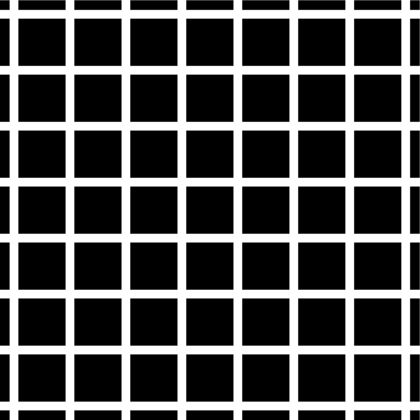 |
|---|
| The Hermann grid illusion |
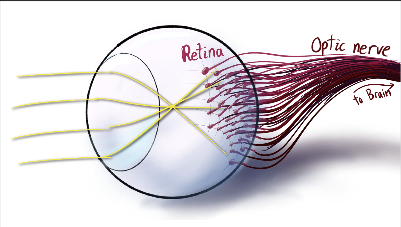
To start, we have our basic schematic of how our eyes work. We’ll make this more detailed as time goes on.
|
|---|
| Schematic of the eye-to-brain pipeline |
Light comes in thru the eye’s lens, and projects onto the back wall. This is full of many light-gathering cells called the retina. Each retinal cell sends its information down the optic nerve, plunging into the incomprehensible jumble of neurons and synapses we call the brain.
For some more detail on the retina itself, the light is absorbed by rod and cone cells, and the signal propagates down a few layers of neurons before reaching the optic nerve. (Sidenote, The light actually comes in from the bottom of this diagram, passing thru the nerves and blood vessels before hitting the light-gathering cells. This is hilariously backwards, because it means the optic nerve has to pass through the retina to get to the brain. This is why we have a blind spot. It goes to show, while evolution does create some brilliant structures and solutions, it only finds local maxima. It could accidentally get stuck with all its sensors facing backwards.)
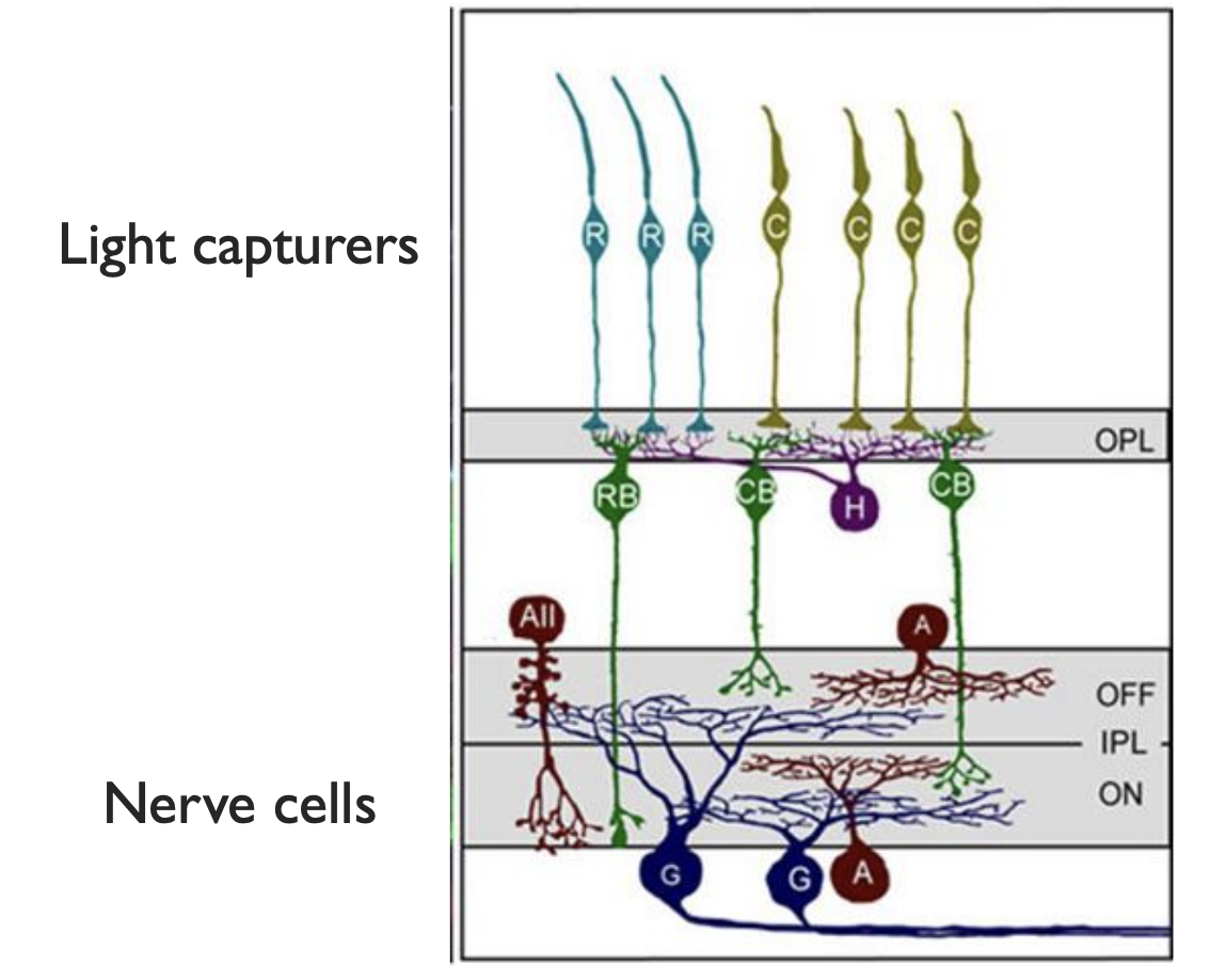 |
|---|
| Close-up diagram of retina |
These few cells show us the first layer of preprocessing, in an effect called Lateral inhibition. Let’s zoom in on one of those horizontal cells, connecting multiple light-gathering cells together.
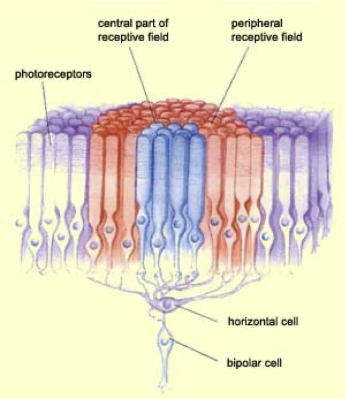 |
|---|
| Diagram of the response of a horizontal cell to adjacent light-gathering cells, showing lateral inhibition. |
The horizontal cell is associated to some point on the visual field. If that point lights up, the horizontal cell activates and the signal goes forth to the brain. If a nearby point lights up, then it inhibits the horizontal cell. In other words, nearby light makes that point look darker. We graph which points around the horizontal cell activate it, and which inhibit it, getting the response field of the neuron. It looks like the figure below.
 |
|---|
| pictorial version of the retina response field |
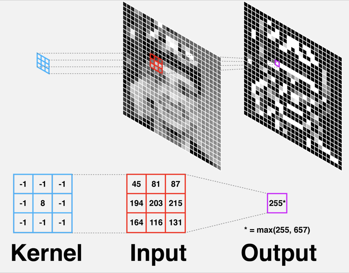
Before the raw data from our retina is sent to the brain, it gets filtered thru the horizontal cells using this function. This is better known as a Convolution filter. If we think of each retina as a pixel, this exactly corresponds with a classic technique in image processing. See the figure below. The response function is the kernel, a window which we center on a point in the image. Looking through the window, some parts are made brighter (the center), and some parts are given negative brightness (the edges), and adding up the result gives the new value for the pixel.
 |
|---|
| Diagram of convolutional filter, From Gregory Gundersen |
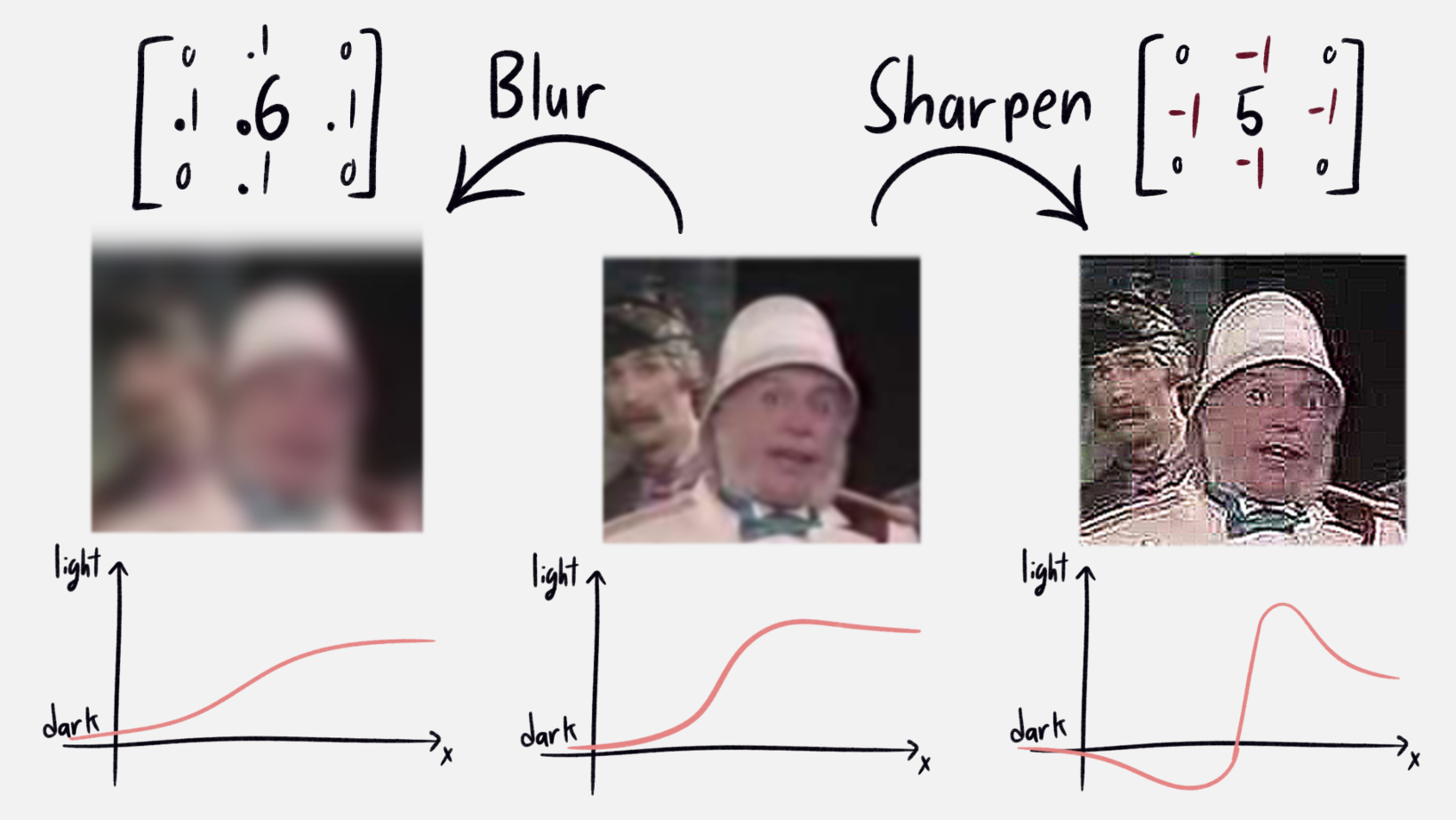
The response field above acts to sharpen the image. To see why, let us start with the conceptually easier bluring kernel. Think about the image as a sandcastle, where the height is the brightness of the associated pixel. To blur the image, you take a little sand from each point and distribute it amongst the neighbors. This knocks pointy parts down a peg, fills in holes, and generally smooths things out. And indeed, convolve the image with the corresponding kernel, and it looks blurrier! In particular, if we look at an edge between a dark and light parts, bluring makes the gradient more shallow (see the image for an example). It softens the edges.
 |
|---|
| Diagram showing effects of blurring and sharpening. |
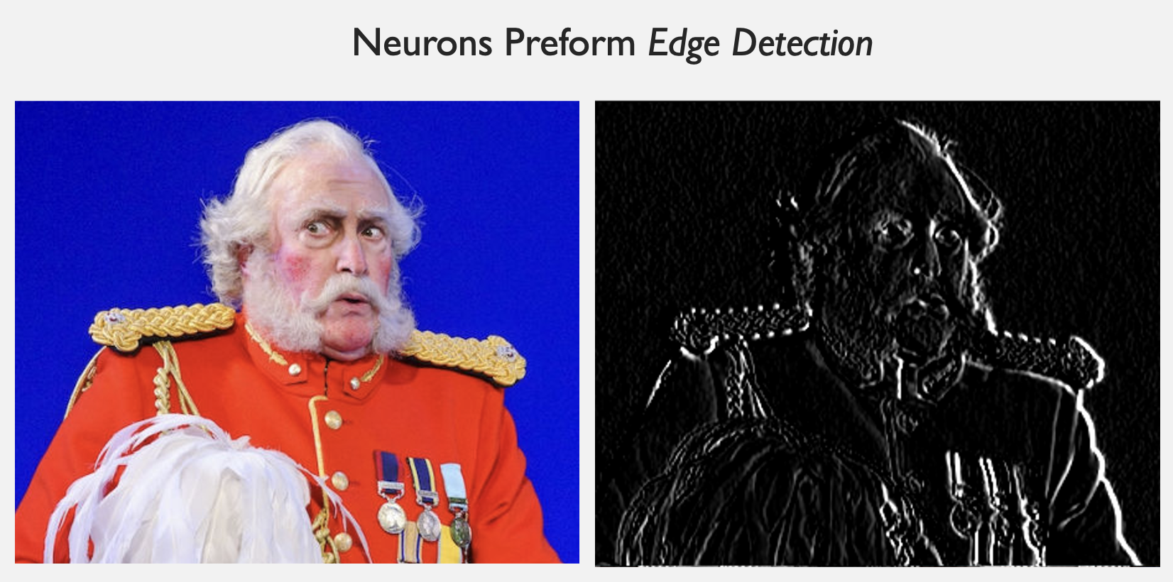
Sharpening is the opposite of blurring. Instead of moving sand from a pile to its neighbors, you pile up sand together, leaving a tall peak surrounded by a moat. Apply this to an edge from dark to light, and we see the light part of the edge gets lighter, while the dark part gets darker. This emphasizes the edge. Applied to a picture, it makes things sharp and vivid. Apply it too much (like i did above), and our modern major general becomes a demon, and the jpeg compression lines become extremely obvious. Like all things, good sharpening is done in moderation.
You see the similarity between the neuron response field above, and the matrix we used for sharpening? This shows the central principle: Lateral inhibition is a hardware accelerated image sharpening filter, built directly into our retina.
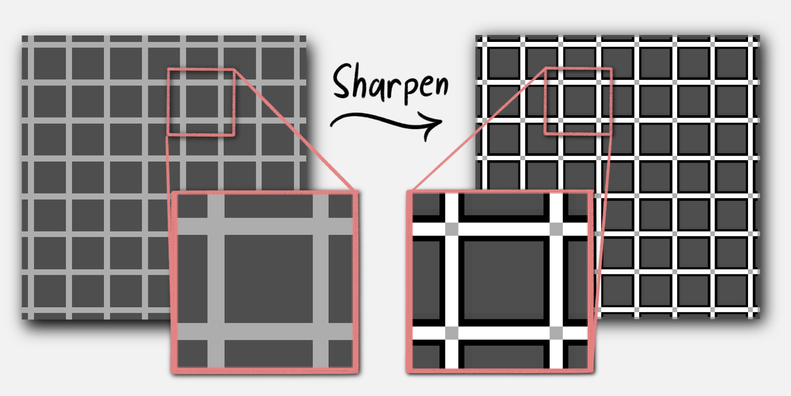
Now let’s go back to that grid. Sharpening lightens the light half of an edge, so a thin bright line becomes brighter. However, there are no edges at the intersection between lines, so there is no brightening. Hence, dark dots! This manifests in usual image processing, as sharpening a grid makes the intersections dark. Therefore, The Hermann grid illusion is an artifact of our retina’s internal sharpening filter
 |
|---|
| Effect of sharpening filter on a grid |
These only appear away from the focus of our vision, where things are blurrier so lateral inhibition is stronger. Disclaimer, As always in biology, this isn’t the whole story. The grid illusion is weaker with wavy lines replacing the grid, implying there is more at play than sharpening.
Contact geometry and the visual cortex.
Here’s another illusion, Kanizsa’s triangle: How many triangles do you see in this picture?
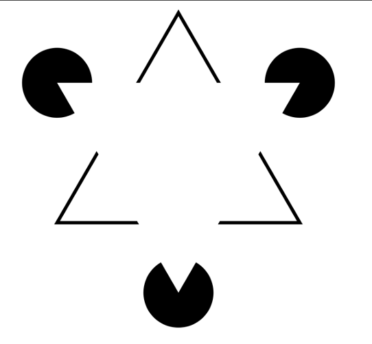 |
|---|
| Kaniza’s triangle, from Wikipedia |
I see two! A broken black one, and an invisible white one. This falls under the umbrella of an Illusory contour, where our brain fills in contours which were never there. Now enters the main character of todays story, the visual cortex.
The signals from our retinas go through the optic nerve into the brain. Their first stop is the visual cortex, a skin a few millimeters thick made of layers of neurons, each applying their own step of image processing. Every point on the retina maps to one on the visual cortex, which then percolates down into the brain proper. From experimental data, the map from the retina to visual cortex preserves angles. That is, it is conformal. This is a bit of a teaser for what to come.
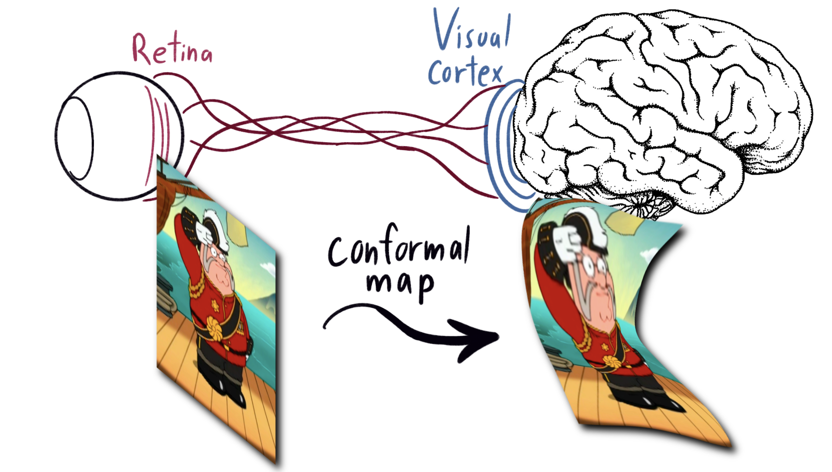 |
|---|
| Diagram showing the map from retina to the surface of the visual cortex, Feat. Peter from family guy dressed as a modern major general. |
Let’s look into the structure of the visual cortex. Here are a trifecta of stains of a cross-section of the cortex, each showing the same neurons in a different way. This picture was drawn by Ramon y Cajal, the father of modern neuroscience. (the visual cortex has a long history of advancing our understanding of the brain.) We have a big spaghetti soup of axons, sorted into clear laters. defined by the type of neurons.
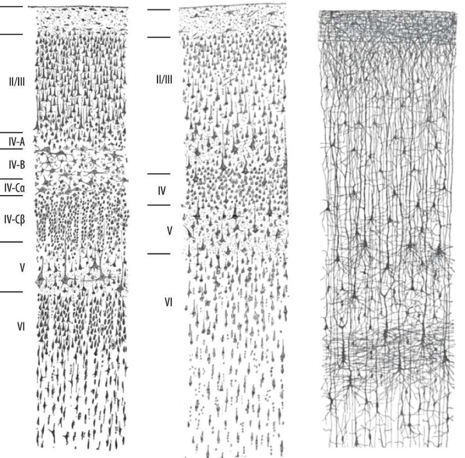 |
|---|
| Drawing of stains of visual cortex, by Ramon y Cajal. From wikimedia |
Just like in the retina, we measure which light causes a neuron to activate, and which makes it deactivate. The leftmost picture below shows the experimental response field. In the middle, we have an idealized approximation, and to the right a 3D graph of the middle function. This acts as the kernel for a new convolution filter. Note how, in the center, the kernel is zero. That is, the neuron does not respond to any direct light, only activating if the signal comes from the right. In our sandpile analogy, this filter moves a little sand into a pile on the right.
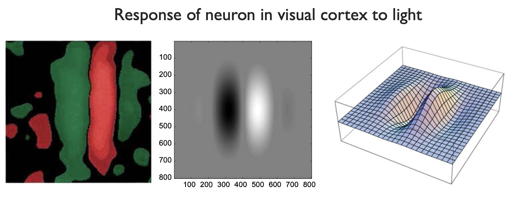 |
|---|
| Response field of neuron in the visual cortex. From Functional geometry of the horizontal connectivity in the primary visual cortex, Sarti et. al |
If we try this for image processing, this kernel effectively measures the \(x\)-derivative of the brightness. So, it detects the rightmost edges of a figure (see below).
 |
|---|
| Result of apply visual cortex response field kernel to image |
But how are these neuron responses oriented? It turns out, their organization defines a couple more structures in the visual cortex. First, the orientation is constant as you move deeper, forming Microcolumns. In Nobel prize-winning work, Hubel and wiesel discovered that the orientation of the columns rotate along a slice of the visual cortex.
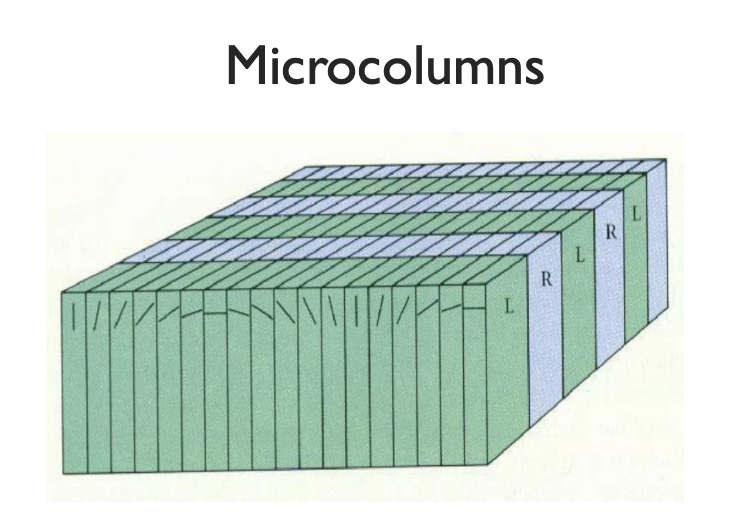 |
|---|
| diagram of microcolumn structure in visual cortex |
Here’s a picture of the orientations of the neurons in the visual cortex
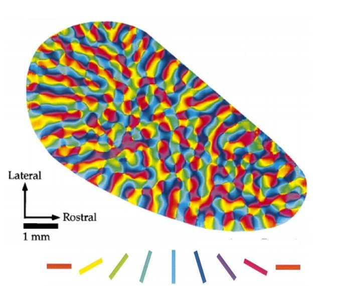 |
|---|
| Orientations of microcolumns in visual cortex. From Orientation Selectivity and the Arrangement of Horizontal Connections in Tree Shrew Striate Cortex |
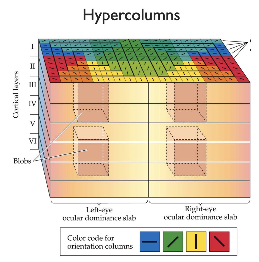
Notice the pinwheel like singularities of the orientation? We use these to organize the visual cortex into another layer of hierarchy, called Hypercolumns. These are comparatively large blocks of the visual cortex with a pinwheel singularity at the center. Suppose we look at a circle: Since the neurons are all edge detectors, the only hypercolumns which activate are on the edge of the circle. Furthermore, only one microcolumn of the hypercolumn will activate, corresponding to the orientation of that edge. Play around with this yourself with this interactive tool.
 |
|---|
| diagram of hypercolumn structure in visual cortex |
We now make a conceptual leap, thinking of hypercolumns as points on the visual field with orientation information. Let us formalize this mathematically. We have the surface of the visual cortex, which we model as a 2 dimensional space \(\mathbb{R}^2\). The space of possible orientations is the space of lines through the origin in 2 dimensional space, which we call \(\mathbb{R}\mathbb{P}^1\). In fact, this is just a circle. So, we model the visual cortex as a 3 dimensional manifold \(\mathbb{R}^2 \times \mathbb{R}\mathbb{P}^1\), with a natural projection to the surface \(\mathbb{R}^2\). This is a continuous model of the discrete pinwheel points.
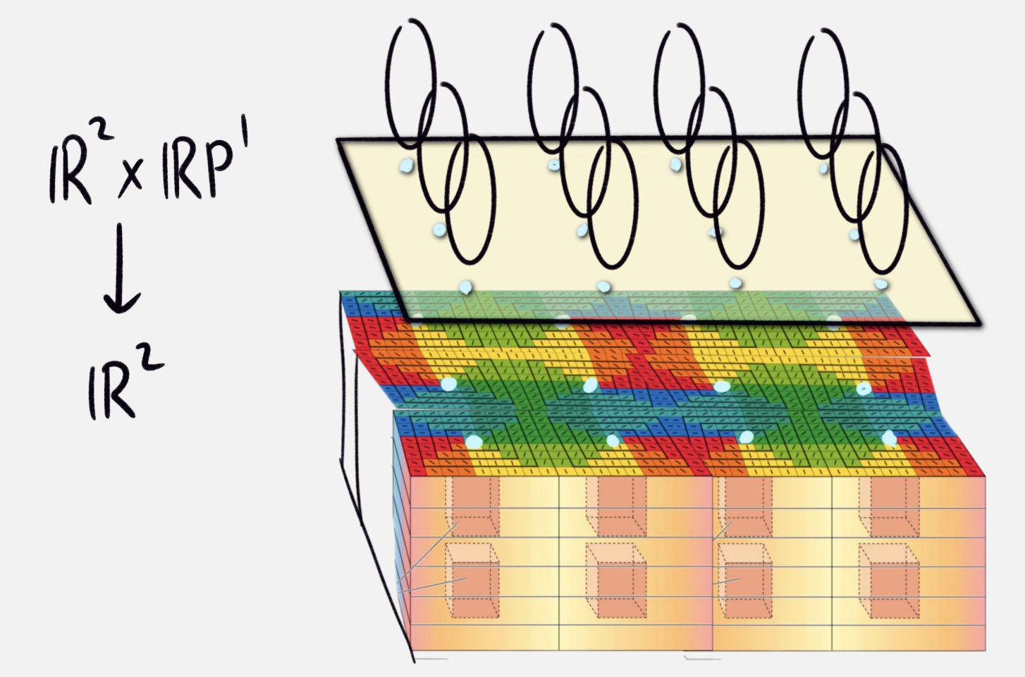 |
|---|
| diagram of 3 manifold associated to hypercolumn structures |
This gives our brain a nice way to interpret shapes. Look at a circle again. Our brain selects the edge automatically, the position and angle of each part selecting a point in our three dimensional manifold \(\mathbb{R}^2 \times \mathbb{R} \mathbb{P}^1\). The edge of the circle lifts to a path, which spirals around the third dimension. Any path in \(\mathbb{R}^2\) lifts to \(\mathbb{R}^2 \times \mathbb{R} \mathbb{P}^1\) in a similar way.
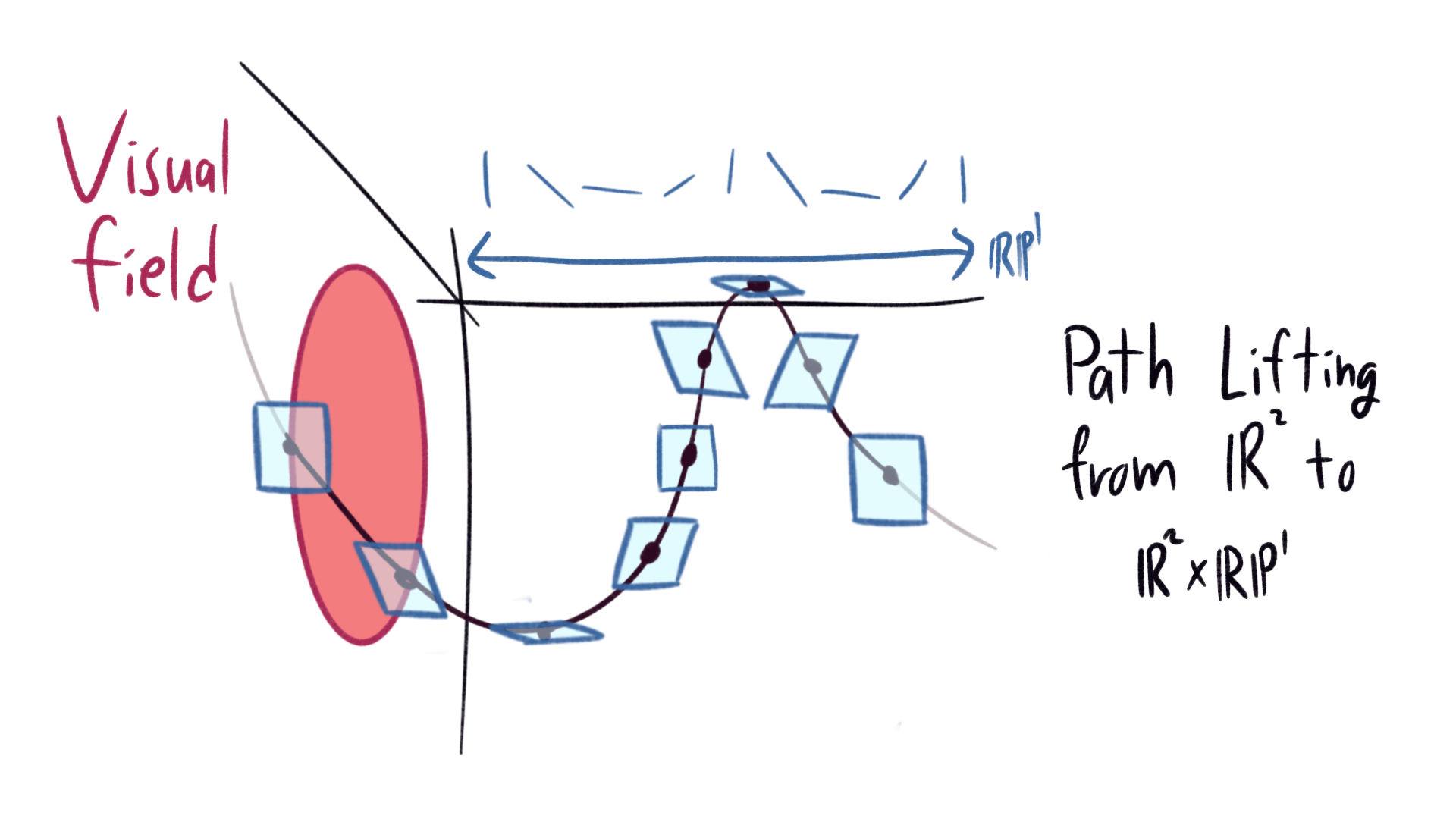 |
|---|
| Lifting from an edge in the visual field to a path in the associated 3-manifold |
We want to think about everything intrinsically inside of our three manifold \(\mathbb{R}^2 \times \mathbb{R} \mathbb{P}^1\), which leads us to ask: What paths in \(\mathbb{R}^2 \times \mathbb{R} \mathbb{P}^1\) are lifts of paths \(\mathbb{R}^2\)? Choose coordinates \((x,y,\theta)\) of \(\mathbb{R}^2 \times \mathbb{R} \mathbb{P}^1\). If a path \((x(t),y(t),\theta(t))\) is a lift from \(\mathbb{R}^2\) that passes through a point \((x(0),y(0),\theta(0))\), then we know the velocity \((\dot{x}(0),\dot{y}(0))\) must have angle \(\theta(0)\). In fact, this is the only restriction. velocity vector of a lifted path in \(\mathbb{R}^2 \times \mathbb{R} \mathbb{P}^1\) has to lie in a two dimensional plane, which twists as \(\theta\) increases. Here’s a picture:
 |
|---|
| Contact structure, formed by 2-planes which rotate as \(\theta\) increases |
We can build this contact structure ourselves with the help of yoga. Hold your elbow to your side, with your arm sticking forward at a right angle, palm towards your body. Then, extend your arm, rotating as you go until your arm is fully extended, and your palm faces down. Your hand just traced out these two planes!
This arrangement of 2-planes is very twisty, so very twisty that one can never realize it as the tangent planes of a 2-dimensional submanifold. Such arrangements are called Contact structures. These arise in math as an odd dimensional version of symplectic geometry, the geometry of classical mechanics. The contact structure above is essentially the standard contact structure on \(\mathbb{R}^3\). Visual contours lift to paths tangent to these 2-planes, which are called Legendrian paths.
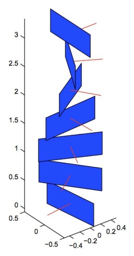
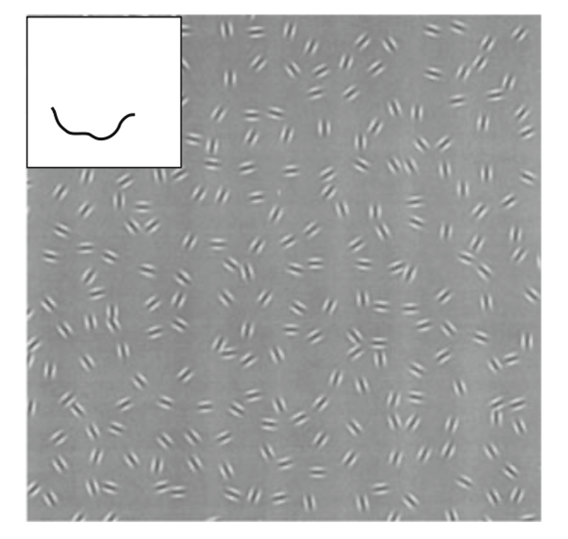
This contact structure helps us connect broken paths. Take the example below. Can you find the continuous path of little blobs through the noise, each lined tip to tail? How does our brain do that? Each little blob has a position and an orientation, so they correspond to a point on \(\mathbb{R}^2 \times \mathbb{RP}^1\). Now our brain just tries to connect the dots, associating points which can be connected with short paths that follow the contact planes. When we minimize the lengths, we get the perceived path, which mathematically is a Legendrian geodesic.
 |
|---|
| Can you find the path of aligned blobs amongst the noise? |
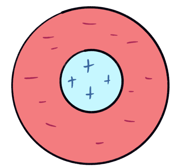
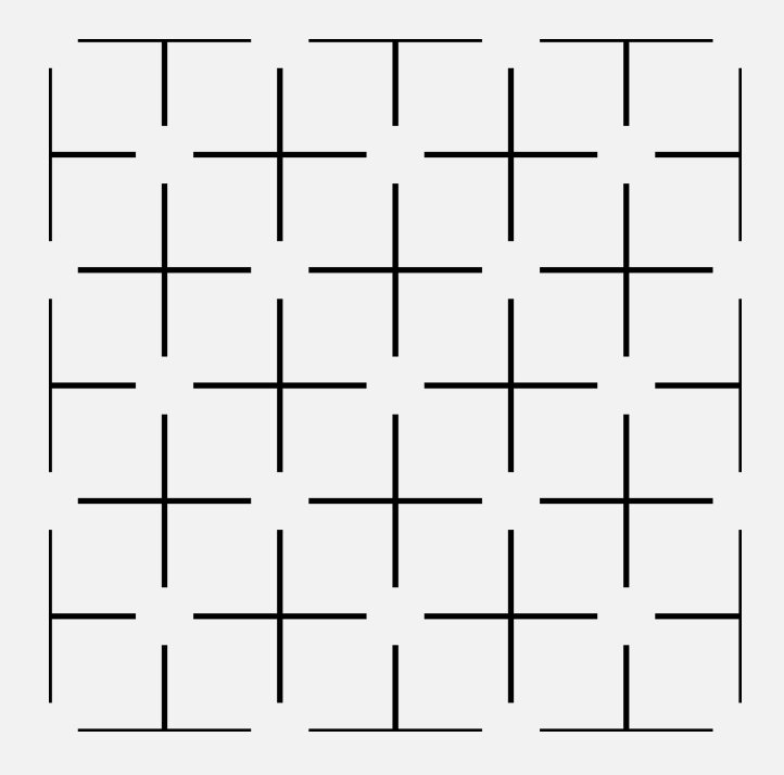
This is the basis for the illusionary contour illusion: The brain converts the image into points in \(\mathbb{R}^2\) points in the contact 3-manifold \(\mathbb{R}^2 \times \mathbb{RP}^1\) with geodesics tangent to the contact structure. We perceive these connected paths in the original image. For example, in the image below, the four tips of adjacent plusses connect into a little circle.
 |
|---|
| Another instance of illusory contours |
Seeing lie algebras: The symmetries of the visual cortex
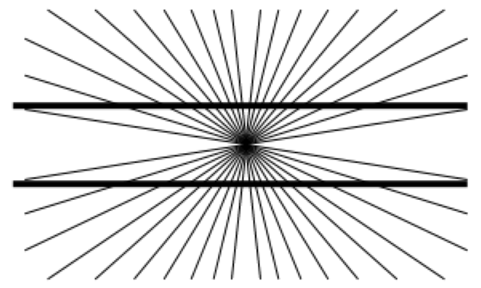
Illusion time: Stare at the center of this starburst for 20-30 seconds (until your eyes start to get tired, and things look a little weird). Then switch to a blank wall. What do you see?
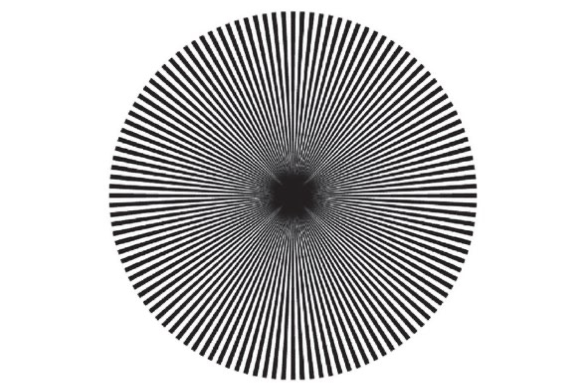 |
|---|
| Stare at the center for 30 seconds, then switch to a wall |
I see a shimmering series of concentric circles in the periphery. It belongs to a family of other illusions, each formed by staring at an image of many thin lines in a pattern. The “afterimage” consists of shimmering lines perpendicular to the first. Interestingly, they only appear for certain classes of regular patterns. These illusions were first described by Mackay. I want to describe a later theory of Hoffman, which explains these illusions using the intrinsic geometry of the visual cortex.
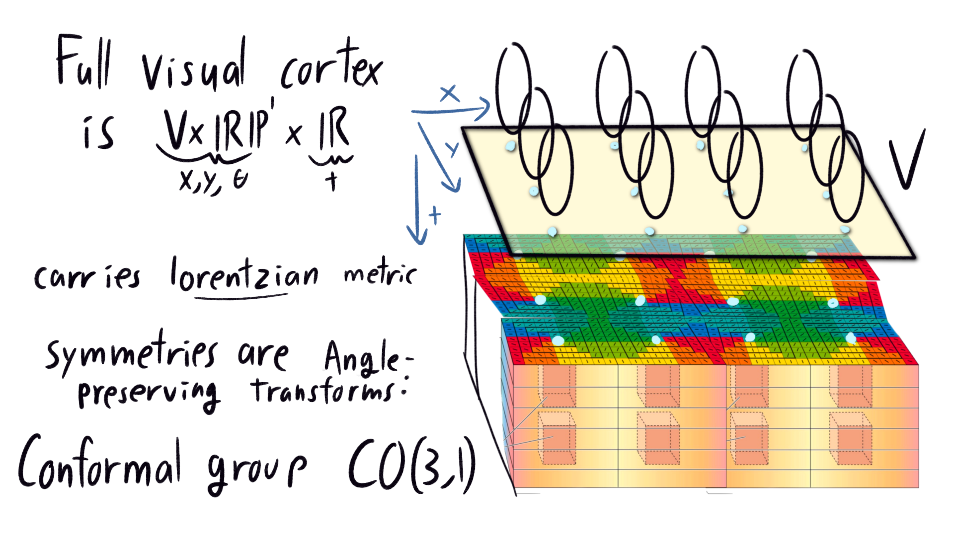
Recall our geometric model of the visual cortex surface as the visual field \(V = \mathbb{R}^2\) times the space of orientations \(\mathbb{RP}^1\). The full visual cortex has many layers, so our manifold should really get an extra dimension: a four dimensional manifold \(V \times \mathbb{RP}^1 \times \mathbb{R}\).
 |
We think of this new depth dimension as time. This makes sense because signals propagate at a finite speed through neurons: Only about 2 m/s in the visual cortex. The image from the retina takes some time to percolate down the visual cortex. As the image moves down, new images from later time are sent to the top. The visual cortex has a whole time series of pictures falling through.
We endow the four-dimensional manifold \(V \times \mathbb{RP}^1 \times \mathbb{R}\) with a metric which looks like spacetime. Choose coordinates \((x,y,\theta,t)\) such that the length of an infinitesimal vector is \(\text{d} x^2 + \text{d} y^2 +\text{d}\theta^2 - \text{d}t^2\), We demand that, locally, symmetries of the visual cortex 4-manifold preserve angles, where angles are measured using this weird metric. These are called conformal transforms, and the set of all such transforms forms the group \(CO(3,1)\) (where \(3\) is the number of positive length directions, and \(1\) is the number of negative length directions). This is a nice 15 dimensional Lie group, with very explicit descriptions of each element. (Note that \(CO(3,1)\) are only local symmetries, and we don’t need that these symmetries extend globally to the whole four-manifold. Mathematically, we describe this best with a principle \(CO(3,1)\)-bundle, or its associated adjoint bundle.)
I’ve made a lot of assumptions without justification, like the group of symmetries that we allow, or the signature of the metric. We have biology to thank for these. Beautifully, each of generators of \(CO(3,1)\) correspond to distortions of the visual field coming from a change of perspective. A single object, if oriented or moved differently, looks very different as a cascade of images falling down the visual cortex. We want to perceive all these signals as the same object, so our perception should be invariant under these distortions. This justifies the group \(CO(3,1)\), and hence the negative sign in the metric. Another piece of evidence comes from the map between the retina and surface of the visual cortex, which was experimentally measured to be conformal. A conformal map is necessary to ensure that the conformal group \(CO(3,1)\) lifts from symmetries of the visual field.
Let me describe some visual transforms coming from moving an object around, and their associated subgroups of \(CO(3,1)\). First, translation! moving an object horizontally or vertically across your visual field comes from the map \((x,y)\to (x+a,y+b)\) for some constants \(a,b\). This is certainly conformal. Likewise, rotating an object in your visual field is rotation of \((x,y)\), another subgroup of \(CO(3,1)\). Or, we could move an object closer, which makes it scale up in our visual field. This relates to the subgroup of dilations in \(CO(3,1)\). Here’s a table of the other correspondences
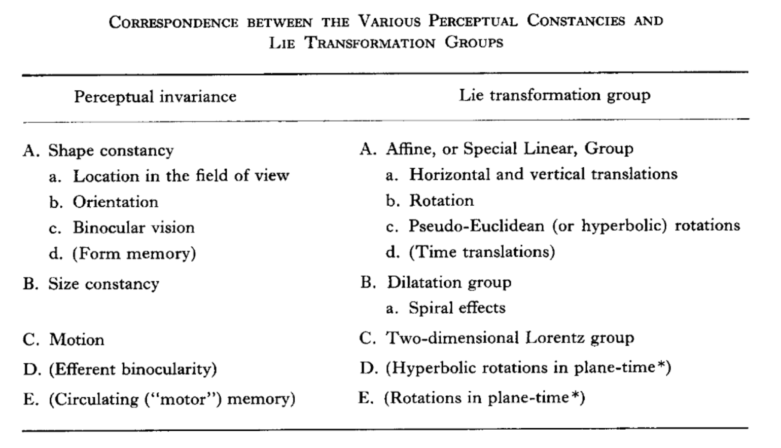 |
|---|
| Table corresponding distortions of the visual field due to changing perception with subgroups of \(CO(3,1)\). From The Visual Cortex is a Contact Bundle |
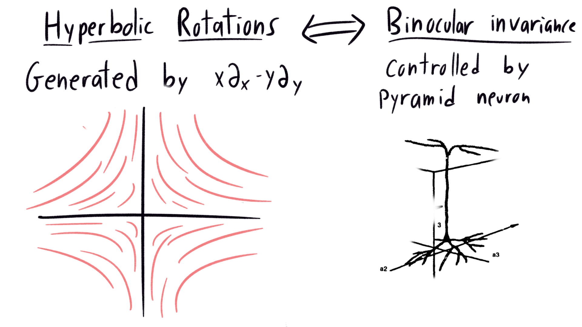
Here are some highlights. An interesting spatial effect comes from binocular vision. When incorporating two, spaced apart eyes into a single visual field, we necessarily introduce some distortions. For example, hold your finger at arms length between your fingers. Keeping focus with both eyes, move it to just before your nose. Right between your eyes, you see more of both sides of your finger. If we convert that to a single image, the finger necessarily becomes wider, while remaining the same height. Binocular vision makes things near your face squash vertically and expand horizontally, which is called a hyperbolic rotation. Though this isn’t conformal in \(x,y\), its lift to \(\theta\) will be conformal.
The hyperbolicness might seem rather far fetched, but it’s quite natural with the right framework. While single-eye, cyclopean vision looks like a surface of a sphere, binocular vision naturally carries hyperbolic geometry! (For example, the level sets of distance look like circles, like a horocycle in hyperbolic geometry)
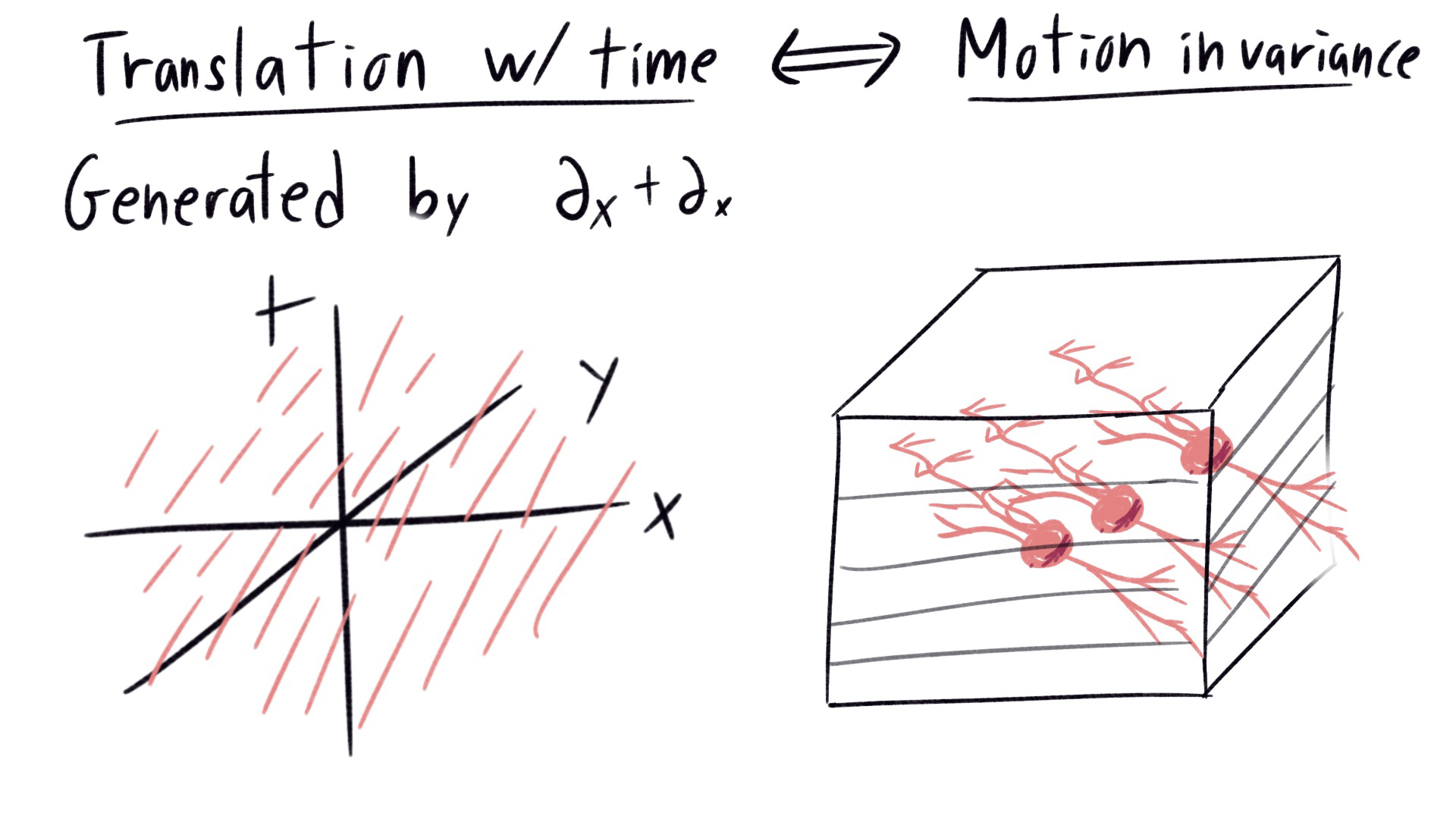
Finally, there are conformal transforms involving time. For example, consider an object moving with a constant velocity. This is generated by translation in both space and time, which is also a conformal transform of \(V\times \mathbb{RP}^1 \times \mathbb{R}\), acting on both the space \(V\) and time coordinate \(\mathbb{R}\).
neuron shapes and lie algebras
We know now that we want our perception to be invariant under the conformal group \(CO(3,1)\). But how does our brain go about that? One hint comes from the development of human perception. Newborns do not intuitively grasp that an object held far away and the same object held close are the same. They only begin to perceive objects scale-invariantly after 36-48 weeks. This change coincides with the addition of a new type of neuron to their visual cortex pallets, the stellate neuron. Somehow, the stellate neurons provide scale-invariant perception.
Infinitesimally, the scaling action is generated by a vector field which points radially outward. On the left of the image below, we show a few orbits of this action: Its like zooming through a snowstorm in your car. On the right, we have a diagram of the stellate neuron, which with axons radiating symmetrically out from a central body. What do you notice about the pictures? Do they look similar?
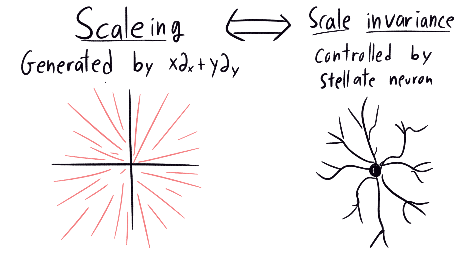 |
|---|
| Correspondence between lie group orbits of scaling, and the neuron responsible for perceptual invariance under scaling |
This incredibly leading question should be confusing, insulting even. Like, how could the shape of the neuron possibly have anything to do with the orbits of this vector field? Here’s the version of the above question from Hoffman’s paper:
It is difficult for anyone versed in the qualitative theory of differential equations to gaze upon such Golgi-Cox preparations of cortical neurons without being reminded of a local phase portrait.
C’mon man, you don’t have to patronize me :( Anyway, one way to make our perception scale-invariant is to simulate what our visual field looks like, scaled up. We scale the visual field up by all possible amounts and add the resulting images together, and the signal to our brain is the same no matter the starting scale. But there’s trouble in the neighborhood, because scaling (and other transforms) require integrating a vector field into a flow. If we only let neurons connect with their neighbors, the signal can only be modified with local changes. In effect, local connections only simulate differential operators. So how do we integrate a vector field?
In comes the stellate neuron, overseeing the neighborhood like the homeowners association. It receives a signal, and expands it radially symmetrically to a whole host of new neurons, scaling up the signal. In other words, The axons of the stellate neuron simulate the flows of the scaling vector field. It’s brilliant: our brain couldn’t make a computer to scale up the image, so instead it designed built in hardware. Let’s see a couple more examples.
Consider hyperbolic distortions of the visual field, which arise due to binocular vision. The orbits of the hyperbolic distortions are hyperbolas, seen on the left. On the right, we see the pyramid neuron responsible. On top, it gathers data from the vertical (in visual space) direction, then it sends outputs to the horizontal direction at the bottom. From the top down, the axons look like simulated hyperbolas.
 |
|---|
| Correspondence between lie group orbits of hyperbolic rotation, and the neuron responsible for perceptual invariance under binocular distortion |
One more. Motion in the visual field comes from translation in both position and time. The orbits are lines in 3 dimensional space. On the right, we see the neurons responsible for the perceptual invariance of neurons. Since each slice of the visual cortex captures a different time, a neuron passing across layer compares the visual field at different times. We see that the neurons responsible for motion invariance are roughly linear, in the same direction as the translation. These cells act like motion detectors, firing whenever an object moves in a specified direction at a point in the visual field.
 |
|---|
| Correspondence between lie group orbits of translation in both space and time, and the neuron responsible for perceptual invariance under motion. Note that the neurons are horizontally mirrored from intended, sorry :( |
In fact, we have neurons for every generator of the lie algebra of \(CO(3,1)\).
Some illusions
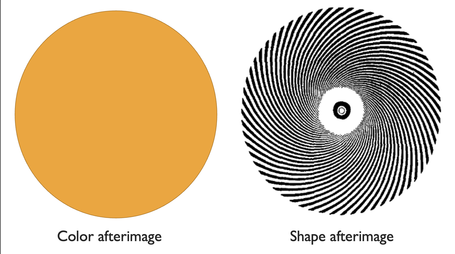
These lie-algebra neurons, if properly abused, let us see lie algebras. This is what underlies the illusion from the beginning of this section. We saw a type of after-image. Start by taking a look at the orange circle on the left, staring at the center for ~20 seconds, or until your eyes get weird and tired. Then, switch to a blank wall. What do you see? I see the orange circle turn blue – an afterimage.
 |
|---|
| Afterimage illusions for both color and shape. |
This happens because our orange neurons get tired from too much orange. Switch to a white wall, and everything lights up except the orange. We are left with anti-orange, which is blue! The same thing happened with the radial lines. Stare at them for too long, and your scaling neurons fire and fire and fire until they just tuckered out. Switch to a blank wall, and we’re left with anti-radial, which is concentric circles! We are seeing a shape-afterimage, instead of a color one.
Now try this with the spiral to the right. What shape afterimage do you see? what direction does it go? I see another spiral moving the opposite direction. The spiral arises from a linear combination of two effects, a scaling and a rotation. The resulting after image is the opposite combination of these same effects. In general, an alternating pattern of curves forming an orbit of \(CO(3,1)\) will produce an after-image with perpendicular curves.
Now what about our motion example, which incorporates time with space? Well, stare at the center of this moving thingy for 20-30 s (I promise I won’t hypnotize you). Then, look around. What do you see?
| Stare at the center for 30s, then look around your surroundings. From Wikipedia |
https://en.wikipedia.org/wiki/Motion_aftereffect
I see disconcerting distortions, it looks like the center of my visual field expands while the peripherally contracts. This In the center, our “move in” neurons got tired, so things look like anti-moving inwards. In other words, they expand out! This reminds me of waterfalls. After staring at a waterfall for a while, it looks like the center of my vision is rising. This illusion is usually called a motion aftereffect
Another neat fact: these illusions add together linearly. If you alternate between two patterns, then the resulting afterimage is the vector field sum of the afterimages of each of the patterns. Or, you could lay one illusion on top of another:
 |
|---|
| Illusion where straight lines appear curved when superimposed over radial lines. |
This picture consists of a central family of radial lines, and to parallel black lines. Do the black lines look parallel to you? to me, they seem to bulge outwards. when our scaling detectors get tired, and we see the parallel lines, we observe a smaller radial component. this bows the parallel lines out!
Summary: The geometry of the visual cortex
We have talked about quite a few different geometric structures adapted for vision by evolution:
- The Retina has built in image sharpening neurons
- The visual cortex has built in edge detectors, which we mathematically model using contact geometry
- The symmetries of this contact geometry represent the distortion of the visual field (in space and time) under a change in perspective
- To ensure our perception is invariant under change of perspective, our brain includes neurons shaped like the orbits of a symmetry, to mechanically simulate the changing of perspective. This explains our very first game, where we could tell if two shapes were the same without conscious thought. The visual cortex uses lie-algebra shaped neurons to ensure that the rotated shapes enter the brain with nearly identical symbols. This preprocessing converts the visual field into a collecting of abstract shapes, existing irrespective of location or orientation. These shapes are fed to the brain, mise en place, fully prepared to be mused about and mulled over.
Finally, there’s one more way to probe the visual cortex. Hallucinations! When we close our eyes, and no light gets in, we still see patterns appearing from the darkness. These look like faintly colored dots, moving wavefronts, whole scintillating grids of light, etc. These so-called phosphenes come from many sources, but a big one is the visual cortex itself. Your brain is constantly pulsing, with plane waves propagating across the surface. As they pass the visual cortex, we perceive the waves as vision. Some patterns are especially present, the form constants. These include spirals, concentric rings, radial lines, etc. Sound familiar? These are exactly the orbits of the symmetry groups, the shapes for which we have explicitly designed neurons.
Try this yourself! Cover your eyes, and for a couple minutes, really pay attention to what you see. If you’d like to cheat, you can close your eyes really hard or press lightly on them with your hands. This makes many more patterns show up, but its through physically stimulating your retina, rather than the visual cortex. (incidentally, this is why people “see stars” when they get smacked.) If you really wanna see, take some DMT or another hallucinogen. DMT makes the serotonin flow freely, which makes neurons more likely to activate each-other across the board. This makes the usual quiet babble of the brain froth up, strengthening the traveling waves and making much flashier hallucinations. Combined with an altered state of mind which is very good at ascribing meaning to things, and you have a potentially spiritual experience. Or you could, you know, just get really tired and rub your eyes.
References:
- The Visual Cortex is a Contact Bundle, by W. Hoffman
- This is mainly about the role of contact geometry, but also has a bunch of discussion of the symmetries of the visual field
- The Lie algebra of visual perception by W. Hoffman
- This is purely about the lie algebra symmetries of the visual cortex, and has a whole section explaining different illusions
- What Geometric Visual Hallucinations Tell Us about the Visual cortex, by Bressloff et. al
- Talks about the hallucinations and their relationship with visual cortex geometry.
- Elements of Neurogeometry: Functional Architectures of Vision, by Petitot
- Book about the subject I outlined here. A lot more focus on the signal analysis aspects and the contact geometry, no mention of the Lie group symmetry things.