Toric structure on the complex projective plane

Feb 2026

CP2 blog

Summary:

A point in the complex projective plane can be described by a triple of complex numbers, each described by a magnitude and a phase. Forgetting the phase defines a map from $\mathbb{CP}^2$ to a triangle, whose fibers are tori. Here is a collection of visualizations of this toric structure.

To visualize a high dimensional manifold, we must cut down dimensions until we have a 2 dimensional object living in 3D. The two main techniques for this are projecting and slicing. Projecting shows a low dimensional shadow of the high dimensional object, while slices show the fibers under some projection. Stacking slices next to one another implies higher dimensions. I would like to visualize the complex projective plane $\mathbb{CP}^2$, which is a four dimensional manifold. There is a map $\mu:\mathbb{CP}^2 \to \RR^2$ whose image is a triangle $\Delta$. The fibers of $\mu$ slice $\mathbb{CP}^2$ into 2 dimensional tori. This picture shows the projection to the triangle and the slicing into tori all at once:

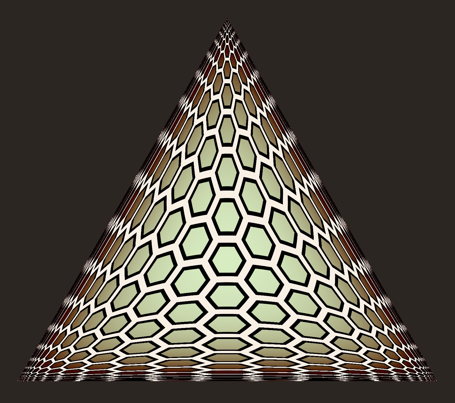
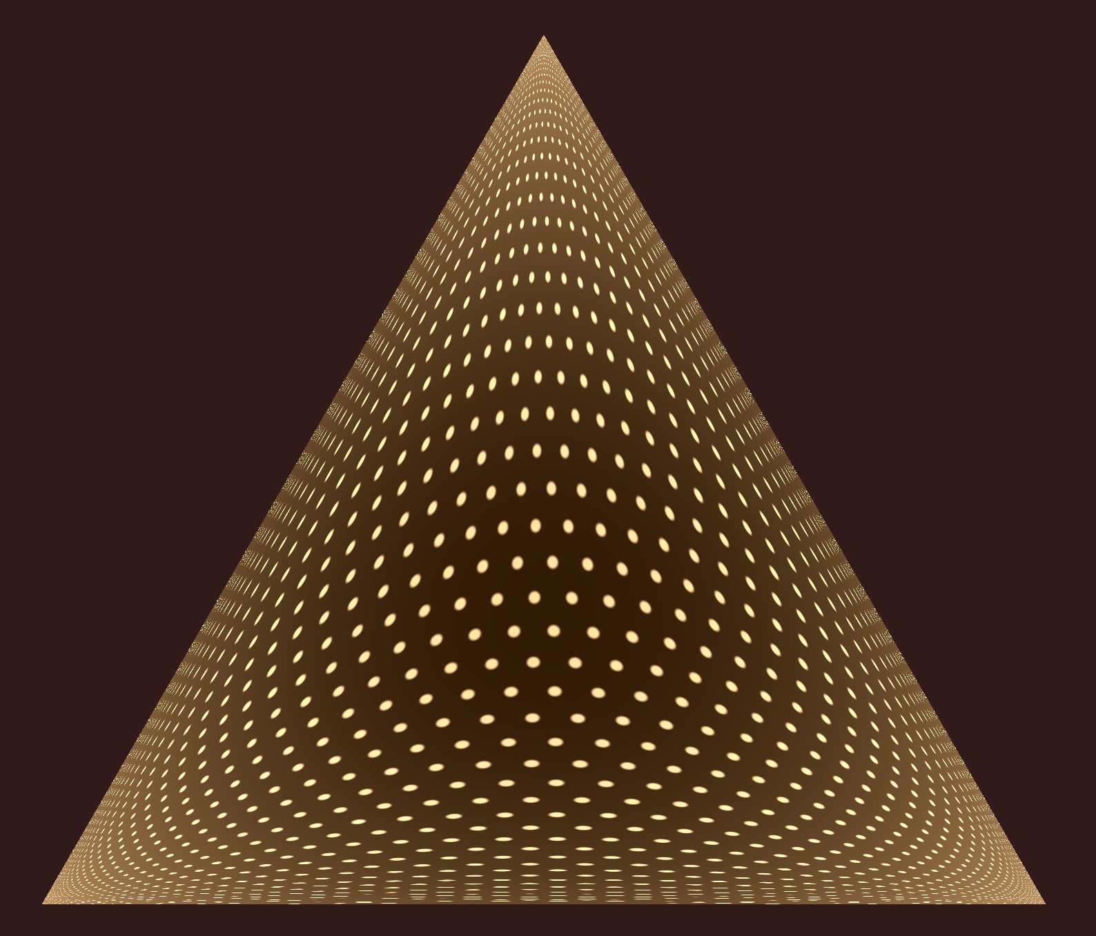
the toric tortoiseshell

A distorted hexagonal tiling illustrating the topology of $\mathbb{CP}^2$

Imagine identifying the opposite edges of each hexagon, to form a torus. This picture shows a family of 2 dimensional tori parametrized by a triangle, which traces out a four dimensional manifold. However, as we near the edges of the triangle, the tiles degenerate into lines. The associated tori degenerate into circles. On the corners, the tiles (and thus the tori) degenerate into points (see picture below). All together, we get a topologically nontrivial four manifold without boundary, the complex projective plane $\mathbb{CP}^2$.

Toric structure on $\mathbb{CP}^2$

Folding up the hexagons makes a torus fibration over the triangle $\Delta$ with the topology of $\mathbb{CP}^2$.

This decomposition of $\mathbb{CP}^2$ into families of tori is called a toric structure. We should think of this like a four-dimensional manifold of revolution, where we revolve around two separate axes. In this post, I’d like to explain the toric structure on $\mathbb{CP}^2$ and how I made this image.

Toric structures

The toric structure on $\mathbb{CP}^2$ is defined by isolating the phase and magnitude of the coordinates of a point in projective space. In particular, we will define a map from $\mathbb{CP}^2$ to a triangle $\Delta$ using only the magnitude. The fiber over each point will be a torus of possible phases. It is easiest to introduce these ideas on the simpler 4-manifold, the complex plane $\mathbb{C}^2$.

Toric structure on $\mathbb{C}^2$

The complex plane $\CC^2$ is built out of tori similarly to the complex projective plane. A point in $\CC^2$ is a pair of complex numbers $(z_1,z_2)$. Consider the map $\mu: \CC^2 \to \RR_{\geq 0}^2$ defined by taking the magnitude squared of each number

The fibers of $\mu$ are pairs of complex numbers with prescribed magnitude, which are defined by a pair of phases. Generically, these are two dimensional tori called the Clifford tori:

However, some of the fibers are lower dimensional tori. If $r_1 = 0$, then $z_1=0$ and the fiber $\mu\inv(0,r_2^2) = (0,r_2 e^{i \theta_2})$ is a circle. Likewise, if $r_2=0$, the fiber is the circle $(r_1 e^{i \theta_1},0)$. Finally, if $r_1=r_2=0$, then the fiber is simply the origin, $\mu\inv(0,0)= 0$. The structure of the fibers is summarized in the figure below.

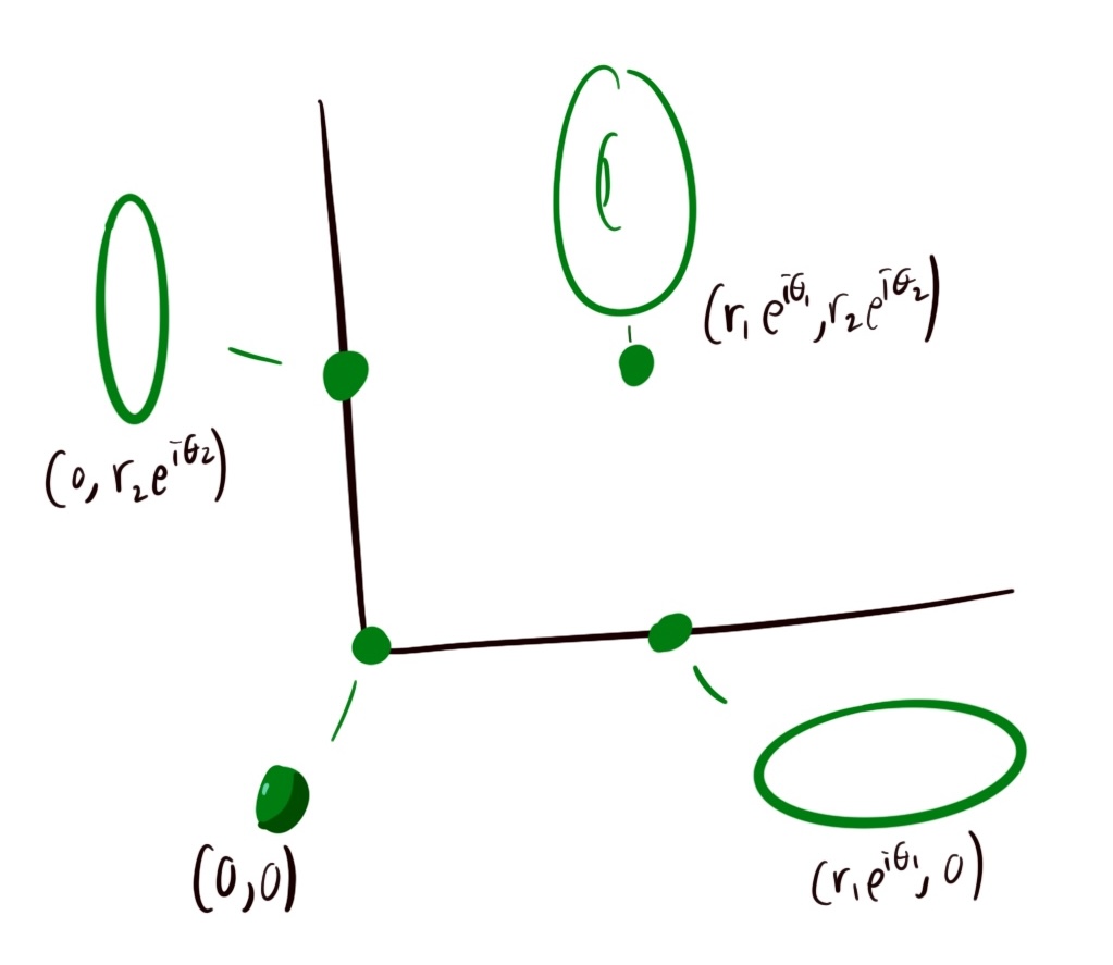
$\CC^2$ as a torus fibration over the positive quadrent

To illustrate the degeneration of the tori, we unwrap the tori into rectangles with the opposite sides identified. As the torus moves to the y-axis, the rectangle collapses onto a vertical line. At the x-axis, the rectangle collapses to a horizontal line. At the origin, the rectangle degenerates to a point. The behavior of the rectangle is encoded in the following picture. Identify the opposite edges of each square, and we get a family of tori over $\RR_{\geq 0}^2$ with the topology of $\mathbb{C}^2$.

Rectangles on $\RR_{\geq 0}^2$ illustrating the toric structure of $\mathbb{C}^2$.

Toric structure on $\mathbb{CP}^2$

Let $[z_0:z_1:z_2]$ be a point in $\mathbb{CP}^2$ in projective coordinates. Take the norm squared of each coordinate to get the point $(\vert z_0\vert ^2,\vert z_1\vert ^2,\vert z_2\vert ^2)$, which lives in $\RR_{\geq 0}^3$, the positive orthant of $\RR^3$ (map 1 in the figure below). The projective coordinates are only well defined up to scaling, so we need to identify points $(x,y,z) \sim (\lambda x, \lambda y, \lambda z)$ for $(x,y,z) \in \RR_{\geq 0}^3$ and $\lambda \in \RR_{>0}$. It is most convenient to chose a representative, by scaling the $(x,y,z)$ to like on the plane $x+y+z=1$ (map 3 in the figure below). Define the “Toric moment map” $\mu$ by

The image of $\mu$ is the intersection of $\RR^3_{\geq 0}$ with a plane, which is a triangle. Choosing coordinates on the plane, we get a map $\mu:\mathbb{CP}^2 \to \RR^2$ with image any fixed triangle $\Delta$(map 4 in the figure below). Succinctly, $\mu([z_0,z_1,z_2])$ is the point $(\vert z_0\vert ^2,\vert z_1\vert ^2,\vert z_2\vert ^2)$ in barycentric coordinates of $\Delta$.

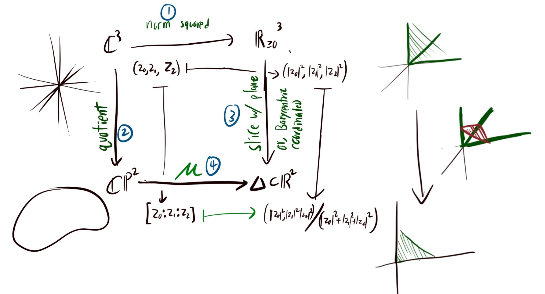
The maps in the definition of the toric moment map $\mu$.

For a point $\vec{x} = (r_0^2,r_1^2,r_2^2)$ in the interior of $\Delta$, the preimage $\mu\inv(\vec{x})$ consists of the points \([r_0e^{i \theta_0} : r_1 e^{i \theta_1}: r_2 e^{i \theta_2}] \in \mathbb{CP}^2\) We have three parameters $(\theta_0,\theta_1,\theta_2) \in U(1)^3$. But we must divide out by the scaling action on $\CC^3$:

Therefore, the pre-image $\mu^{-1}(p)$ is the quotient of $U(1)^3$ by the diagonal subtorus $U(1) \subset U(1)^3$. The result is a two dimensional torus $T^2$.

When $p$ moves to the edge of the triangle, the torus degenerates. We can see this in an affine slice. The coordinates of the affine slice $\CC^2$ provide a natural choice of triangle, with vertices ${(0,0), (0,1), (1,0)}$. The affine slice covers the complement of the hypotenuse. When point $p$ lies on the $y$-axis, any point in the preimage has $r_1=0$. One circle $r_1 e^{i\theta_1}$ degenerates to a point, so the preimage is the remaining circle $r_2 e^{i\theta_2}$. Likewise, when $r_2=0$, the circle the premiere is the circle $r_1 e^{i \theta_1}$. As $r_1=r_2=0$, the preimage is the point $0$.

Choosing different affine charts, we perform a similar analysis for all edges of the triangle. The preimage above any interior point of $\Delta$ is a 2-torus, the preimage of any point on the interior of an edge of $\Delta$ is a circle, and the pre-image of a vertex of $\Delta$ is a point.

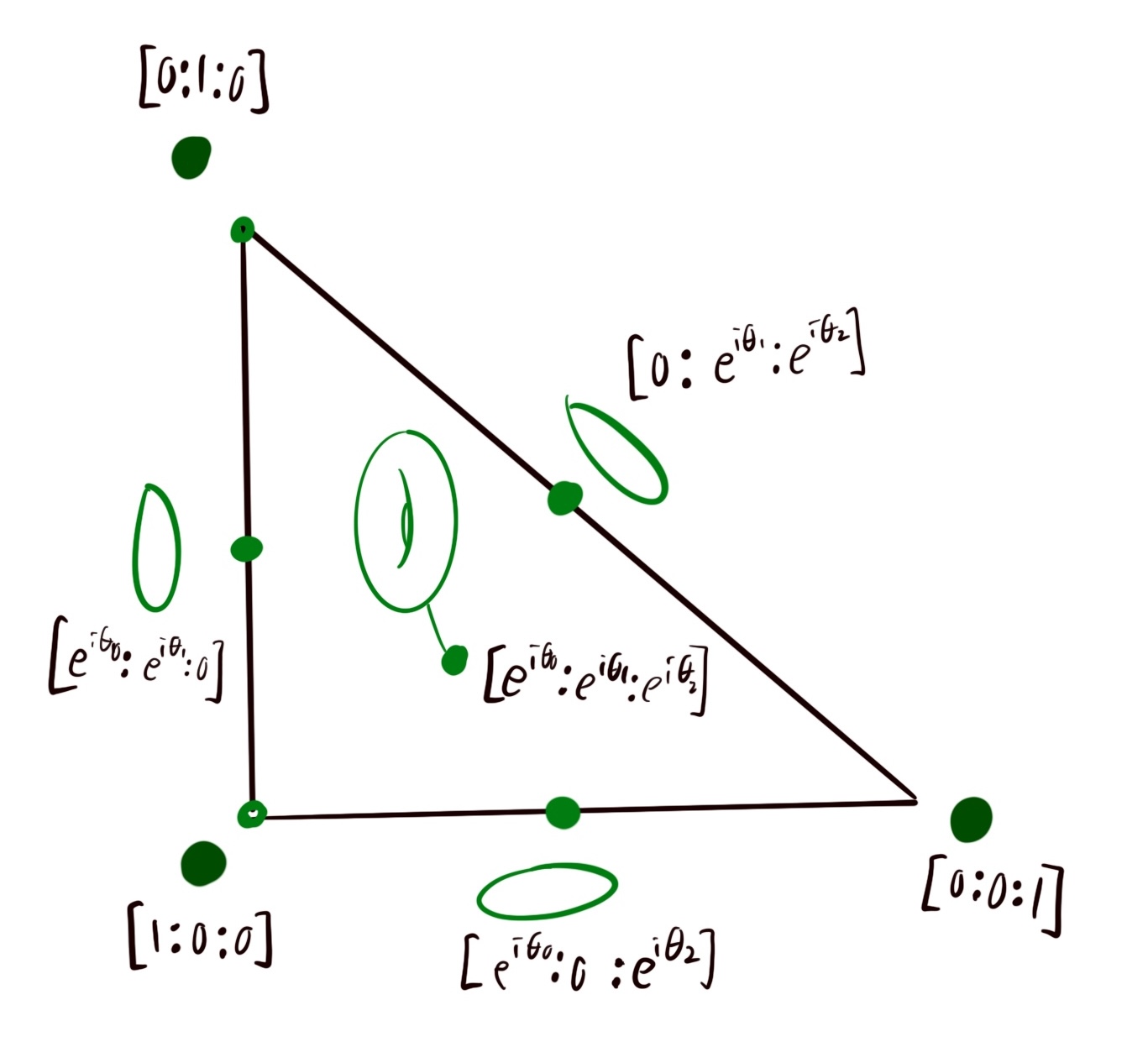
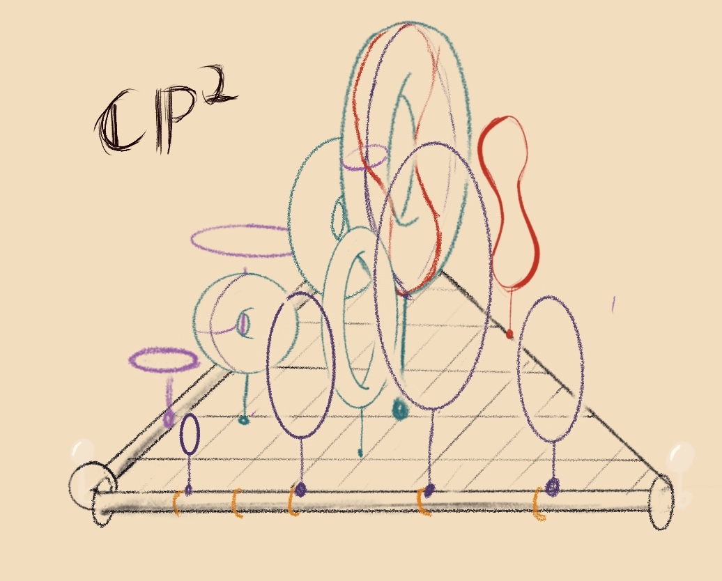
Cartoon of the fibers of $\mu : \mathbb{CP}^2 \to \Delta$.

The three sides of the triangle degenerate the central torus into three different quotient tori. This is best understood by thinking of the torus as a square with edges identified. The vertical edge shrinks the $(1,0)$ subtorus, meaning we lose the $x$-direction. The horizontal edge degenerates the $(0,1)$ torus, losing the $y$ direction. The diagonal degnerates the $(1,1)$ subtorus which is generated by a line with slope 1.

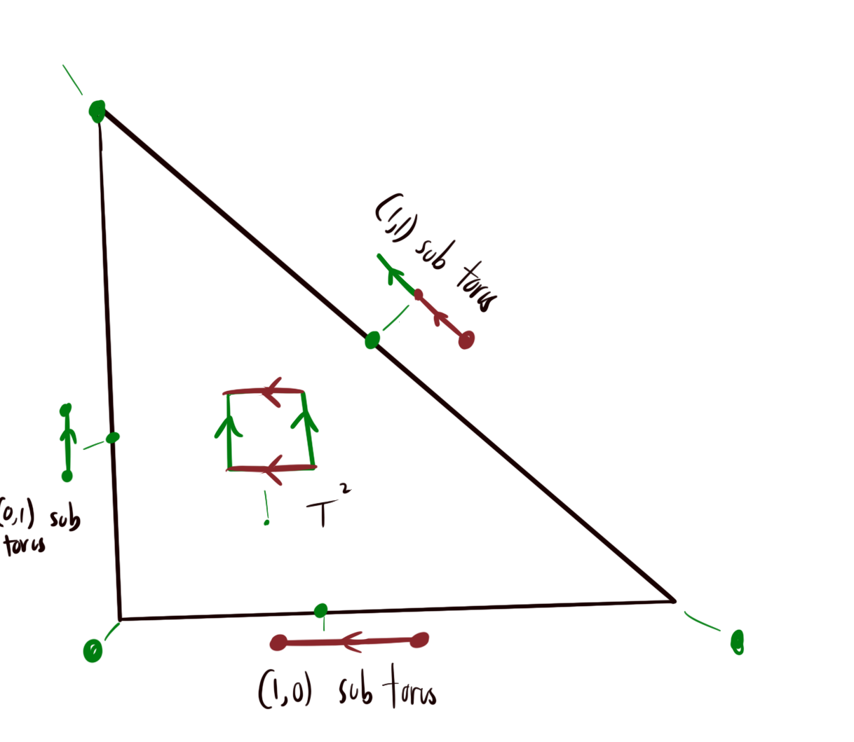
Cartoon of the toric fibration on $\mathbb{CP}^2$, with tori rendered as squares with their edges identified.

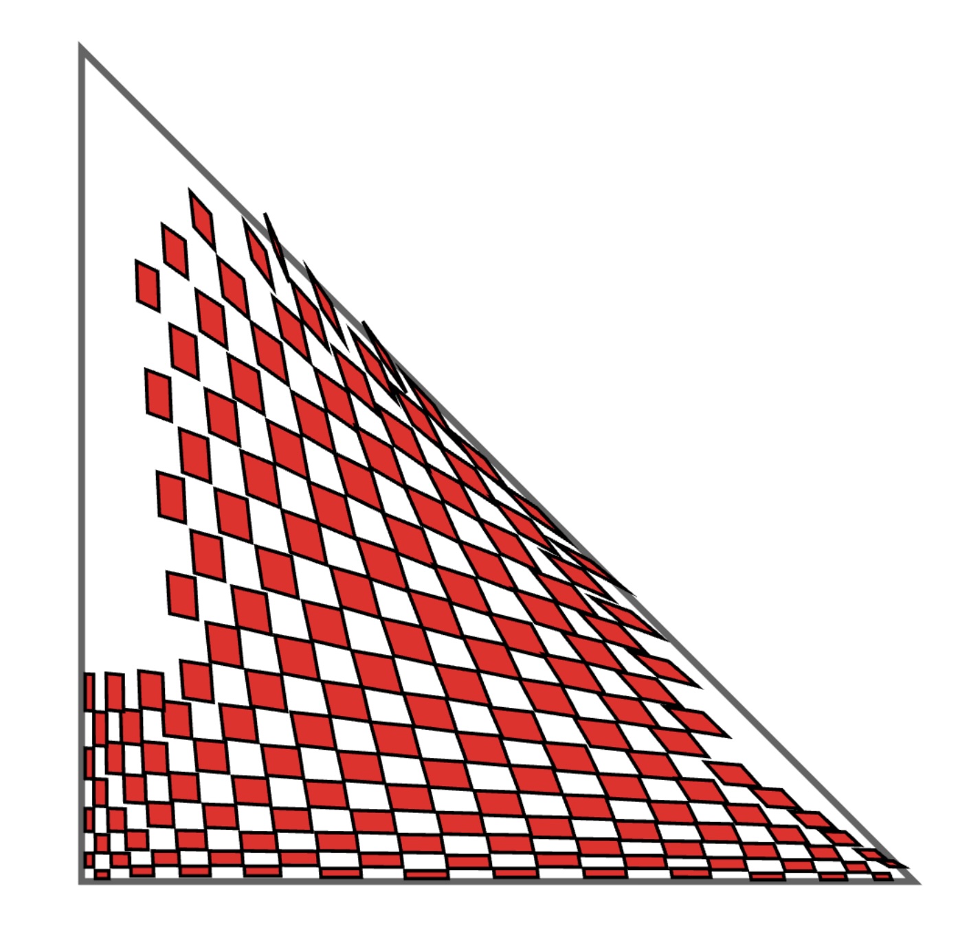
Here are the unfolded tori on the triangle, showing how they degenerate as they move to the boundary.

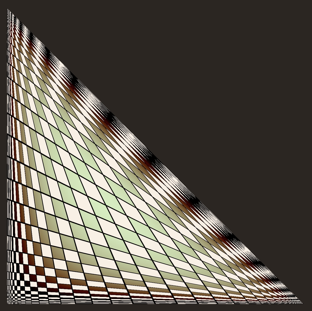
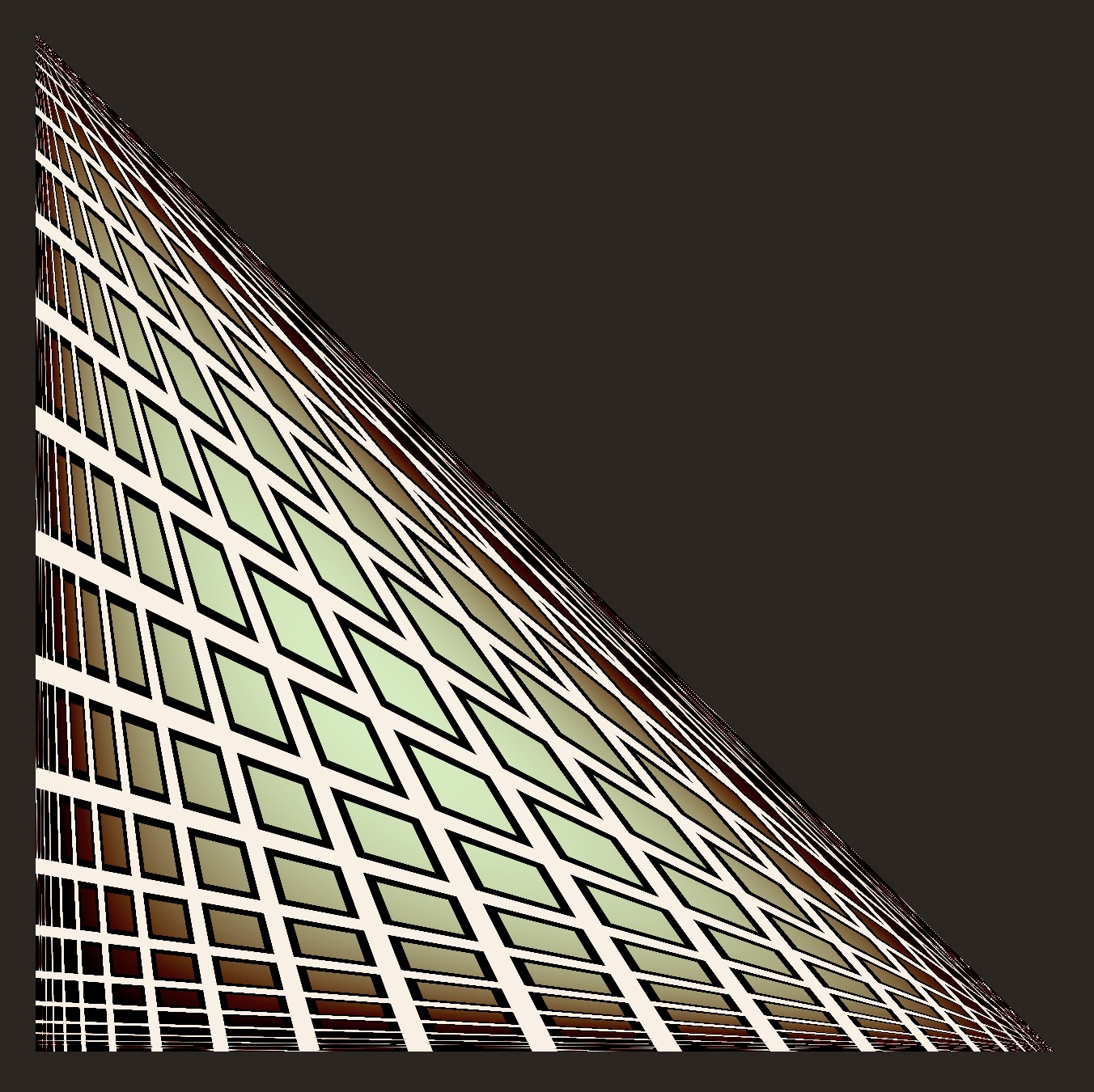
Tori living on a triangle

Two figures showing how the tori on a triangle degenerate at the edges to form $\mathbb{CP}^2$. On the left, a the unfolded tori form a checkerboard pattern. On the right, every tile is filled in with a gap between adjacent tiles.

The hexagonal turtle shell at the beginning of the section is mathematically the same picture as this. But, we apply an affine transform to make the triangle equilateral, and we render the Voronoi tiling by hexagons instead of the parallelogram tiling. This illustrates the underlying symmetry exchanging the three edges.

Notice that the tile edges form lines which pass to the vertices of the triangle. We should think of this like a 2 point perspective drawing, where the hypotenuse is the horizon and the two vertices on the hypotenuse are the vanishing points. In fact, apply a perspective transform to the checkerboard illustrating the toric structure on $\CC^2$, and we obtain the checkerboard illustrating the toric structure on $\mathbb{CP}^2$ (see below). Fitting that a projective transform of our illustration of a plane gives our illustration of a projective plane.

Making the picture

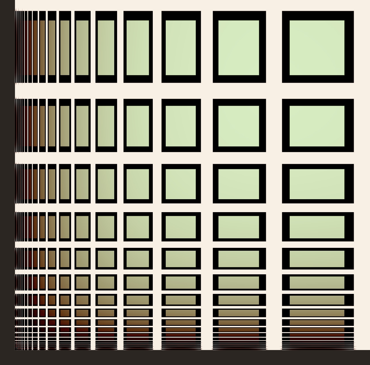
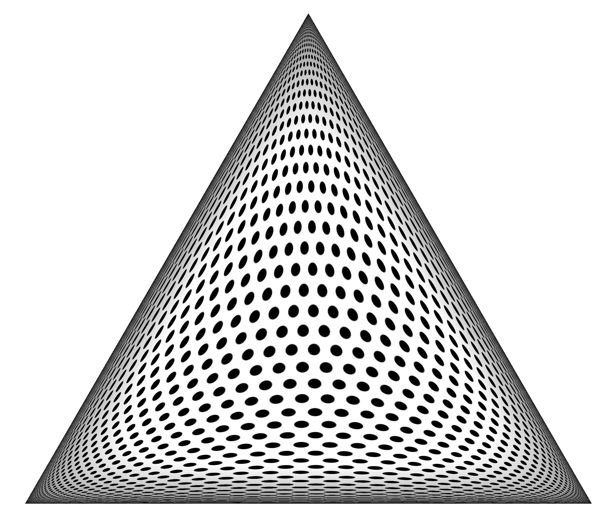
Though I draw the tori as tiles, I think of them as lattices. A lattice $\Lambda \subset \RR^2$ defines a torus $\RR^2 / \Lambda$. The toric structure on $\mathbb{CP}^2$ induces a family of tori on the triangle $\Delta$, which I think of as a spatially-varying lattice $\Lambda(x)$ depending on $x\in \Delta$. We would like to draw $\Lambda(x)$ as a single distorted lattice $\tilde{\Lambda}$. That is, $\tilde{\Lambda}$ is a map from the standard lattice $\mathbb{Z}^2$ to the triangle $\Delta$ which, zooming in near $x\in \Delta$ is nearly periodic. Under a magnifying glass near $x$, $\tilde{\Lambda}$ looks like a rotation or scaling of $\Lambda(x)$. Here is the deformed lattice $\tilde{\Lambda}$ corresponding to the $\mathbb{CP}^2$ pictures in right triangles. Explicitly, for the original lattice $\mathbb{Z}^2 = (n,m)$, the deformed lattice is given in barycentric coordinates as $[e^n,e^m,1]$. In this section, I’ll explain the math and thought process behind this deformed lattice.

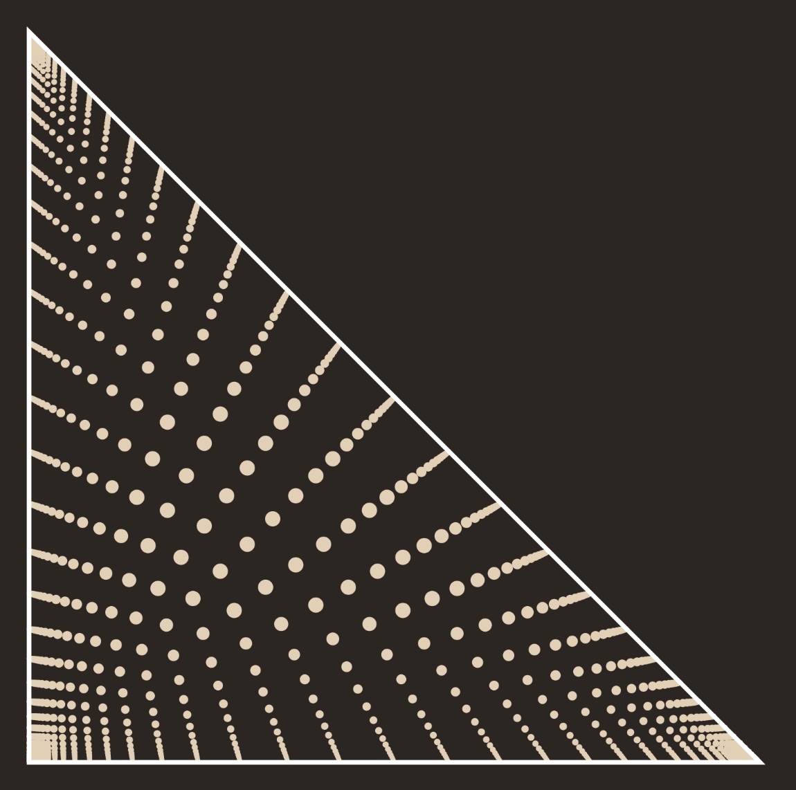
the deformed grid $[e^n,e^m,1]$ in barycentric coordinates. This was used to create the checkerboard patterns above.

One way to produce $\tilde{\Lambda}$ is to find a function $F:\RR^2 \to \Delta$, then define $\tilde{\Lambda}$ as the pushforward of a scaled standard lattice $\tilde{\Lambda} = F(\lambda\mathbb{Z}^2)$. As $\lambda$ becomes smaller, $\tilde{\Lambda}$ becomes finer, and becomes nearly periodic as you zoom in near $x$. More precisely, if $F=(u,v)$ with $u,v:\RR^2 \to \RR$, then near $x$, $F(\lambda \mathbb{Z}^2)$ looks like the lattice spanned by $\langle\nabla u(x), \nabla v(x)\rangle$. To approximate our family of lattices $\Lambda(x)$ with a deformed lattice, we must find functions $u$ and $v$ whose derivatives behave correctly.

Here’s how we want our lattices to degenerate as we move to the edges of the triangle

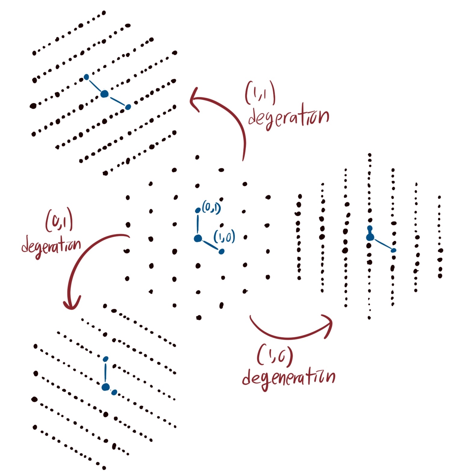
As a lattice degenerates, some of the rows coalesce into solid lines. The three types of degeneration in $\mathbb{CP}^2$ occur when the three directions in a hexagonal lattice coalesce into rows.

Let $\overset{\circ}{\Delta}$ denote the interior of the triangle. For $\tilde{\Lambda}$ to degenerate in this way near the boundary of $\overset{\circ}{\Delta}$ , the inverse function $F\inv: \overset{\circ}{\Delta} \to \RR^2$ must have its derivative go to infinity. We make one more simplification, and define the map $F\inv$ as the gradient of a real valued function

We require $g$ to be a convex function, so that $F\inv: \overset{\circ}{\Delta} \to \RR^2$ is one-to-one. In the language of convex geometry, $F\inv$ is the Legendre transform associated to $g$. The deformed lattice locally defines the lattice spanned by the columns of $\text{Hess } g \inv$. To generate my deformed lattice, I used the following function. Representing a point in $\Delta$ in barycentric coordinates as $(a,b,c)$ with $a+b+c=1$, I define

The graph of this function looks like a pillowcase above the triangular domain.

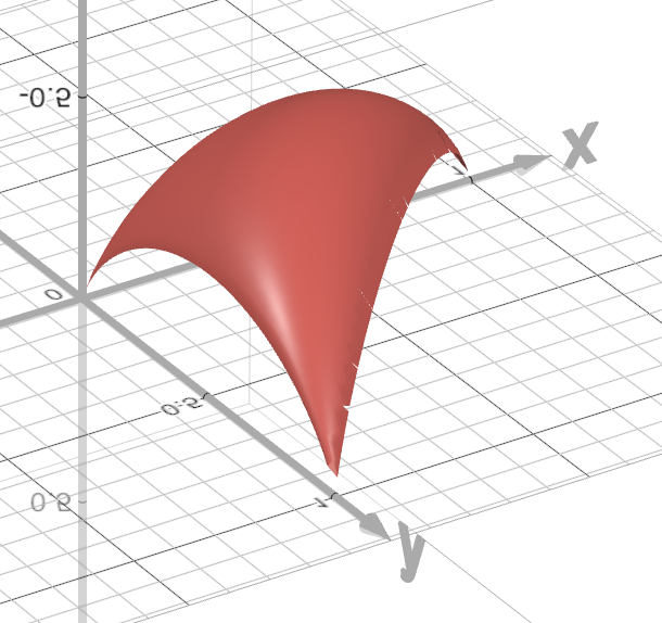
Graph of $g$ plotted above a right triangle.

At the edges of the triangle, the gradient of $g$ diverges. This ensures that $F\inv = \nabla g : \overset{\circ}{\Delta} \to \RR^2$ is 1-1 and onto, so has an inverse. Here’s the resulting grid $F(\mathbb{Z}^2)$:

Deformed lattice illustrating the toric structure on $\mathbb{CP}^2$. For a black and white version, see here.

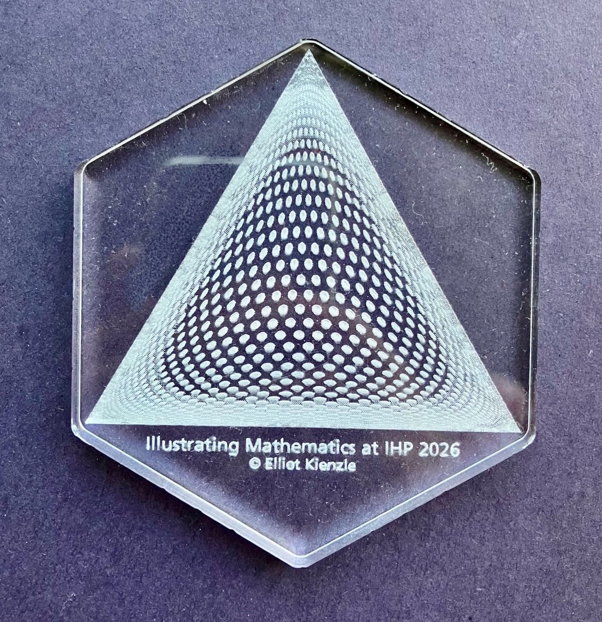
And here is this design, laser etched on acrylic to make a coaster!

Coaster layout and cutout by Edmund Harris.

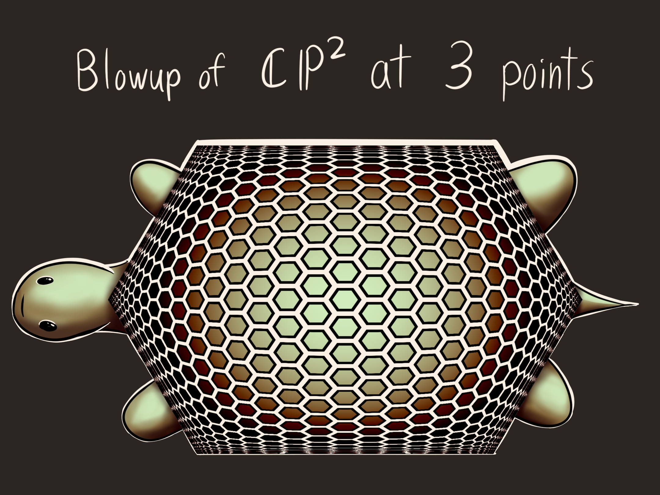
This approach works for any toric variety. For example, we can blow up $\mathbb{CP}^2$ at the fixed points of the toric action to produce a new toric 4-manifold with a new topology. This amounts to chopping off the corners, turning the triangle base into a hexagon. We can illustrate how the torus fibers degenerate at the edges of the hexagon by unfolding the tori into hexagons and decorating the surface. This makes a turtle shell.

He the blowup of $\mathbb{CP}^2$ at 3 points.

Kahler geometry

I got this function $g$ from the paper Kaehler structures on toric varieties by Victor Guilleman. When $g$ is pulled back from $\Delta$ to $\mathbb{CP}^2$, it defines a Kahler potential of the fubini-study form. That is, the complex hessian of the pulled back function gives a hermitian metric which is invariant under the action of $SU(3)$ rotating $\mathbb{CP}^2$. Guilleman provides a similar formula for the Kahler potential of any toric variety.

The map $\mu:\mathbb{CP}^2 \to \RR^2$ is natural with respect to the symplectic form induced by the Fubini-study metric. The hamiltonian vector fields of the $x$ and $y$ functions of $\mu$ commute with one another, and both preserve $\mu$. Therefore, they generate a torus action $T^2 \circlearrowleft \mathbb{CP}^2$ which rotates the torus fibers of $\mu$. This is why we call $\mu$ the moment map. In projective coordinates, this action is given by rotating the phase of 2 of the coordinates

This hamiltonian condition is why we defined $\mu$ using the norm squared of each component, instead of simply the norm.

On a toric Kahler variety, the real torus action extends to a complex torus action. In the case of $\mathbb{CP}^2$, the action by an element of the complex torus $(c_1,c_2) \in (\CC^\ast)^2$ is given by

On a toric variety, there is a single open dense orbit of $(\CC^\ast)^2$. On $\mathbb{CP}^2$, this is the orbit through the point $[1,1,1]$. This is the preimage of the interior of the triangle $\overset{\circ}{\Delta}$ under the moment map.

This parametrizes an open subset of $\mathbb{CP}^2$ by a complex torus $(\CC^\ast)^2 \to \mu\inv(\overset{\circ}{\Delta}) = \overset{\circ}{\Delta} \times T^2$. Using logrithmic coordinates, we can write $(\CC^\ast)^2 = \RR^2 \times T^2$. Explicitly,

The parametrization $\RR^2 \times T^2 \to \overset{\circ}{\Delta} \times T^2$ preserves the phase, so acts as the identity on $T^2$. Therefore, it induces a map $\RR^2 \to \overset{\circ}{\Delta}$, a change of coordinate from the complex torus to the symplectic moment map. Guilleman proved that this map is the Legendre transform associated to the Kahler potential $g$. For exposition, see Kahler geometry of toric manifolds in symplectic coordinates by Miguel Abreu.

This gives the geometric origin of the deformed lattice inside the triangle. It is a lattice in the complex torus $(\mathbb{C}^\ast)^2$, acting on a point in $\mu\inv(\overset{\circ}{\Delta})$ and projected onto $\Delta$. Specializing to $\mathbb{CP}^2$, the lattice in the torus consists of points $(e^{n},e^{m})$ for $n,m \in \mathbb{Z}$, and pushing forward to $\Delta$ results in the points $(1,e^n,e^m)$ in barycentric coordinates.

Finally, the Fubini-Studi metric induces a flat structure on each of the torus fibers. If we respect this flat structure, this defines a spatially varying lattice $\Lambda(x)$ defined over $\Delta$. If we find a deformed lattice $\tilde{\Lambda}$ which locally approximates $\Lambda(x)$, then we could visualize the topology and the metric geometry of $\mathbb{CP}^2$! Unfortunately, though the lattice I use above is qualitatively similar, it doesn’t exactly give the flat metric. I made a set of stamps to try to lay out a metrically correct checkerboard, which you can play with here. Click to place the stamps. Here was my best attempt.

An illustration of the Fubini-study metric. The parallelogram at each point, once opposite edges are glued, gives the flat metric on the torus fiber above that point.