Fubini-Study boot camp

Mar 2024

blog

Summary:

A collection and coalittion of various facts and forms of the Fubini-Study form. I work out the kahler structure of $S^2$ in all of its different coordinates.

Welcome to the Fubini-Study boot camp! For my various needs in life, I needed the details of the Fubini-study form in various coordinates forms. So, I thought I’d compile everything together in one place. Also, this is usually left as an exercise in books, meaning its hard to find guidance if you’re formulae aren’t working. I’ve worked out all the details for the computations here. Perhaps someone else will also find this helpful.

The fubini-study form is the natural Kahler structure on on projective space $\mathbb{C} P^n$. We will think about projective space as $\mathbb{C}^{n+1}\backslash 0$. Later, we will specialize to the case of $\mathbb{C} P^1 \cong S^2$, and compare the projective space coordinates with the other usual coordinates on $S^2$. We prove that the Fubini-study form agrees with the round metric up to a scale. To start, here are the natural coordinates on projective space.

Homogenous coordinates: Identify a point in $\mathbb{C} P^n$ as $[Z_0,\dots,Z_n]$, more succinctly as a vector $\vec{Z} \in \mathbb{C}^{n+1}$. We demand that $\vec{z}$ is not zero, and for every $\lambda \in \mathbb{C}$, we identify $\vec{Z} \cong \lambda \vec{Z}$.

Affine coordinates: We can build coodinate charts on $\mathbb{C} P^n$. Define open sets $U_i$ as the complement of the vanishing locus of the function $z_i$. On $U_i$, we have the coordinate map found by scaling out by $z_i$, and removing the homogenous coordinate 1. $[Z_0,\dots,Z_n] \in U_i \mapsto (\frac{Z_0}{Z_i},\dots,\hat{\frac{Z_i}{Z_i}}, \dots, \frac{Z_0}{Z_n}) \in \mathbb{C}^n$Usually we will work with the affine chart $U_0$, which we identify with points $[1,z_1,\dots,z_n]\in \mathbb{C} P^n$These in bijection with vectors $\vec{z} \in \mathbb{C}^n$.

The fubini-study form

The most natural Kahler form on projective space is the fubini-study form. This takes its most elegant form in projective coordinates: $\omega_{FS} = \frac{i}{2}\partial \bar{\partial } \log \vert Z\vert ^2$ where $\vert Z\vert ^2 = \vert Z_0\vert ^2 + \dots + \vert Z_n\vert ^2$.

Theorem

In affine coordinates, the fubini-study form is

\[\omega_{FS} = \sum\limits_{i,j} \frac{i}{2}\left(\frac{(1+\vert z\vert ^2) \partial ta_{ij} + \bar{z}_i z_j}{(1 + \vert z\vert ^2)^2}\right) \mathrm{d} z_i \wedge \mathrm{d} \bar{z}_j\]

Remark: Notice that the only forms that appear are of the form $\mathrm{d} z \wedge \mathrm{d} \bar{z}$. This ensures that $\omega$ is of type $(1,1)$. This is required for a form to be Kahler.

Proof

We first collect a few computations.

By definition of the change of coordinates, $\vert Z\vert ^2 = 1 + \vert z\vert ^2$
$\partial \vert z\vert ^2 = \sum\limits \bar{z}_i \mathrm{d} z_j := \bar{z} \cdot \mathrm{d} z$, and likewise $\bar{\partial }\vert z\vert ^2 = z \cdot \mathrm{d} \bar{z}$
$\partial \bar{\partial } \vert z\vert ^2 = \sum\limits \partial (z_i \mathrm{d} \bar{z}_i) = \sum\limits \mathrm{d} z _i \wedge \mathrm{d} \bar{z}_i$ Now we compute. For convenience, we will move the constant factors to the other side.

\[\begin{align} \frac{2}{i}\omega_{FS} &= \partial \bar{\partial } \log (1+\vert z\vert ^2) \\ &= \partial \left(\frac{\bar{\partial } (1+\vert z\vert ^2)}{1+\vert z\vert ^2}\right) \\ &= \partial \left(\frac{\bar{z} \cdot \mathrm{d} z}{1+\vert z\vert ^2}\right) \\ &= \frac{\partial (\bar{z}\cdot \mathrm{d} z) (1+\vert z\vert ^2) - \bar{z} \cdot \mathrm{d} z \wedge \partial (1+\vert z\vert ^2)}{(1+\vert z\vert ^2)^2}\\ &= \frac{ \left(\sum\limits_i \mathrm{d} z_i \wedge \mathrm{d} \bar{z}_i\right) (1+\vert z\vert ^2) - \left(\sum\limits_i \bar{z}_i \mathrm{d} z_i\right) \wedge \left(\sum\limits_i z_i \mathrm{d} \bar{z}_i\right)} {(1+\vert z\vert ^2)^2}\\ &= \frac{ \left(\sum\limits_i \mathrm{d} z_i \wedge \mathrm{d} z_i\right) (1+\vert z\vert ^2) - \sum\limits_{i,j} \bar{z}_i z_j \mathrm{d} z_i \wedge\mathrm{d} \bar z_i} {(1+\vert z\vert ^2)^2} \\ &= \sum\limits_{i,j} \frac{(1+\vert z\vert ^2) \partial ta_{ij} - \bar{z}_i z_j}{(1+\vert z\vert ^2)^2} \mathrm{d} z_i \wedge \mathrm{d} \bar z_j\\ \implies \omega_{FS} &= \sum\limits_{i,j} \frac{i}{2}\left(\frac{(1+\vert z\vert ^2) \partial ta_{ij} - \bar{z}_i z_j}{(1 + \vert z\vert ^2)^2}\right) \mathrm{d} z_i \wedge \mathrm{d} \bar{z}_j \end{align}\]

Theorem

IIn projective coordinates, the fubini-study form is

\[\begin{align} \omega_{FS} &= \sum\limits_{i,j} \frac{i}{2}\left(\frac{\vert Z\vert ^2 \partial ta_{ij} - \bar{Z}_i Z_j}{ \vert Z\vert ^4}\right) \mathrm{d} Z_i \wedge \mathrm{d} \bar{Z}_j \\ &= \frac{i}{2}\left(\frac{\mathrm{d} Z \wedge \mathrm{d} \bar{Z}}{\vert Z\vert ^2} - \frac{ \bar{Z} \cdot \mathrm{d} Z \wedge Z \cdot \mathrm{d} \bar Z}{\vert Z\vert ^4} \right) \\ &= \frac{i}{2} \frac{1}{\vert Z\vert ^4}\sum\limits_{i\neq j} \bar{Z}_i Z_i \mathrm{d} Z_j \wedge \mathrm{d} \bar{Z}_j- \bar{Z}_i Z_j \mathrm{d} Z_i \wedge \mathrm{d} \bar{Z}_j \end{align}\]

Remarks:

The second formula is a simple rewriting of the first formula using slicker notation.
Both the numerator and denominator are quartic in $Z$. This ensures the form is invariant under scaling of $Z$, meaning $\omega_{FS}$ descends to a well defined 2-form on $\mathbb{C} P^n$.
As a matrix, $\omega_{FS}$ looks like

$\omega_{FS} = \frac{i}{2} \frac{1}{\vert Z\vert ^4}\begin{pmatrix} \vert Z\vert ^2-\bar{Z}_1 Z_1 & -\bar Z_2 Z_1 & \cdots & -\bar Z_n Z_1 \\ -\bar Z_1 Z_2 & \vert Z\vert ^2-\bar{Z}_2 Z_2 & & \vdots \\ \vdots & & \ddots & \\ -\bar Z_1 Z_n & \cdots & & \vert Z\vert ^n-\bar{Z}_n Z_n \end{pmatrix}$

Proof

For the first formula, this is a word for word rewriting of the proof for affine coordinates, with $1+\vert z\vert ^2$ replaced everywhere with $\vert Z\vert ^2$. The second formula is a rewriting of the first in different notation. We are just left with showing the last formula from the first. Factoring out the common factors of $i/2$ and $1/\vert Z\vert ^2$, this comes from a rearrangement of terms. We need to show

\[\sum\limits_{i,j} (\vert Z\vert ^2\partial ta_{ij} - \bar{Z}_i Z_j )\mathrm{d} Z_i \wedge \mathrm{d} \bar{Z}_j = \sum\limits_{i\neq j} \bar{Z}_i Z_i \mathrm{d} Z_j \wedge \mathrm{d} \bar{Z}_j- \bar{Z}_i Z_j \mathrm{d} Z_i \wedge \mathrm{d} \bar{Z}_j\]

The matrix above was constructed out of the entries of the left side. We need to show the right side gives the entries of the matrix. We split into two cases.

Off diagonal entries ($i \neq j$): The only contribution is $-\bar Z_i Z_j$, which is the desired entry
diagonal entries: The $j$-th diagonal entry is $\vert Z\vert ^2 - \vert Z_j\vert ^2$, which splits as the sum of $\vert Z_i\vert ^2$ for every $i \neq j$ (the $j$ term cancels!) This is exactly the contribution from the right hand side. Therefore, these formulae are the same.

Specializing to $\mathbb{C} P^1$

Coordinates on $S^2$

We start by listing several coordinates on $\mathbb{C} P^1 \cong S^2$.

Projective coordinates $Z \in \mathbb{C}^2$

These are the same coordinates defined for general projective space above. We write $Z = [Z_0:Z_1]$.

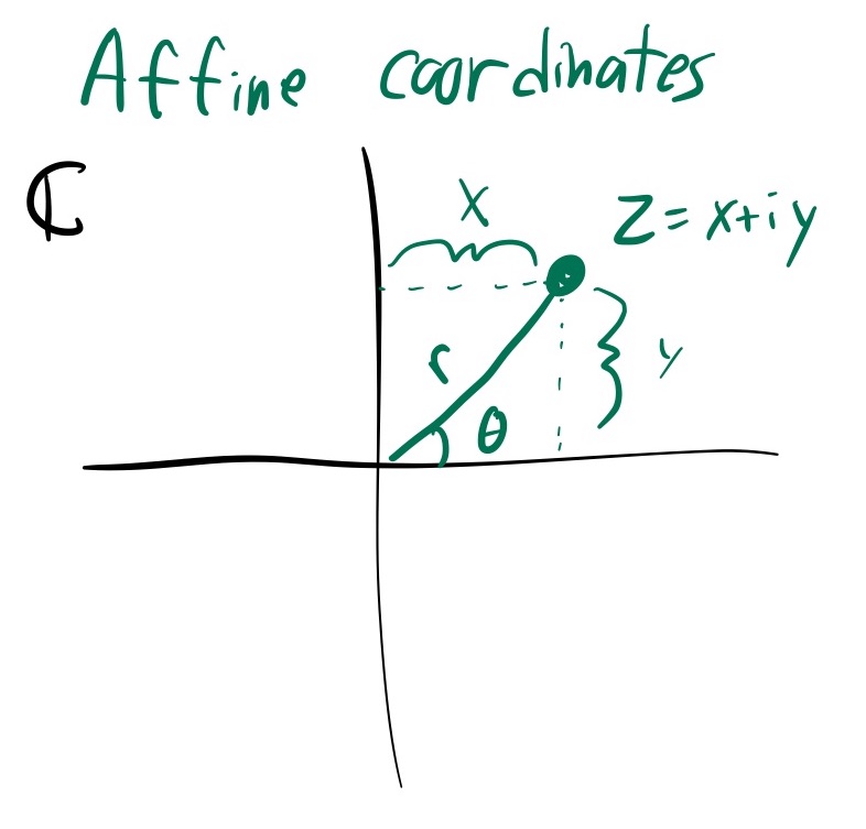
Affine coordinates $z \in \mathbb{C}$, or $(x,y) \in \mathbb{R}^2$

These are the affine coordinates of $\mathbb{C} P^1$ defined above. The real and complex forms relate to eachother by $z = x+iy$.

We also have the polar affine coordinates $(r,\theta)$, defined by $z = r e^{i \theta}$

For future uses, define the function $K = 1+\vert z\vert ^2 = 1 + x^2 + y^2 = 1+r^2$. This is the exponential of the Kahler potential of $\omega_{FS}$, and also the Bergmann Kernel of $\mathbb{C} P^2$.

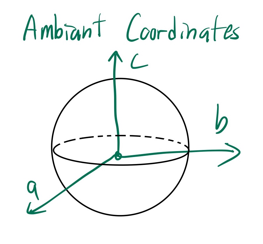
Ambient coordinates $(a,b,c)$

Define the round 2-sphere $S^2$ as the locus of points $(a,b,c) \in \mathbb{R}^3$ such that $a^2 + b^2 + c^2 =1$. We will call $a,b,c$ the ambient coordinates of $S^2$ (We use $a,b,c$ instead of $x,y,z$ to avoid conflict with affine coordinates).

The Kahler potential is $K(a,b,c) = \frac{2}{1-c}$ (proved useing the change of coordinates below)

Toric coordinates $(\theta,h)$

Identify a point on $S^2$ with the azumithal angle $\theta$ and the height $h$, measured in ambiant coordinates.

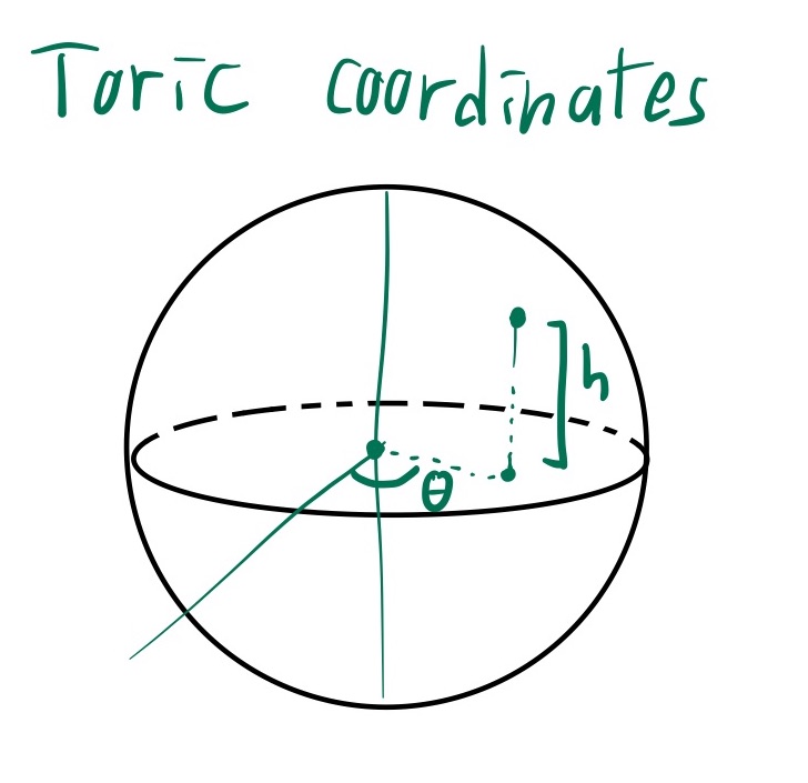
Toric coordinates are essentially cylindrical coordinates $(\rho,\theta,h)$ on $\mathbb{R}^3$. Since the two-sphere has radius 1, we know $\rho^2 + h^2 = 1$. The ambiguity in solving for $\rho$ in terms of $h$ is fixed by the angular coordinate $\theta$. So, $(\theta,h) \in [0,2\pi) \times [-1,1]$ defines a unique point on $S^2$. We should think of toric coordinates as better versions of spherical coordinates, replacing the altitude angle $\phi$ with the height $h = 1-\sin(\phi)$. The formulas are much nicer.

Coordinate transforms

Let me fix notation for changes of coordinates. If I have two sets of coordinates $f_1,\dots,f_n$ and $g_1,\dots,g_m$, say we can write $f$ as a function of $g$. That is, we have formulas $f_i(g_1,\dots,g_m)$. This formula converts us FROM $g$, TO $f$. From this, we can form the Jacobian, which I denote $\mathcal{D}_{(g_i) \to (f_j)}$. For example, say we have coordinates $f_1,f_2,f_3$ and $g_1,g_2$. Then, we define

\[\mathcal{D}_{(g_1,g_2) \to (f_1,f_2,f_3)} = \begin{pmatrix} \frac{\partial f_1}{\partial g_1} & \frac{\partial f_1}{\partial g_2} \\ \frac{\partial f_2}{\partial g_1} & \frac{\partial f_2}{\partial g_2} \\ \frac{\partial f_3}{\partial g_1} & \frac{\partial f_3}{\partial g_2}\end{pmatrix}\]

The numerators are constant along the rows, and the demoninators are constant along the columns. We can read off cool things from this matrix. For example, if we think of the functions $f_i(g_1,\dots, g_m)$ as defining a morphism $\phi:M_g \to M_f$ between the $g$-coordinates manifold to the $f$-coordinates manifold. Then, we have

\[\phi^* \mathrm{d} f_i = \mathrm{d} f_i(g_1,\dots,g_m) = \frac{\partial f_1}{\partial g_1} \mathrm{d} g_1 + \dots + \frac{\partial f_1}{\partial g_m} \mathrm{d} g_m\]

The pullback of a one form $\mathrm{d} f$ is the corresponding row of the Jacobian. Writing a one-form in the basis $\mathrm{d} f_i$ as a row vector, then the pullback from $M_f$ to $M_g$ is right-multiplication of the row vector by $\mathcal{D}_{(g) \to (f)}$.

The vector field $\partial_{g_i}$ pushes forward to a vector field

\[\phi_* \partial _{g_i} = \frac{\partial f_1}{\partial g_i} \partial _{f_1} + \dots + \frac{\partial f_n}{\partial g_i} \partial _{f_n}\]

The coefficients of the pushfroward vector field come from the corresponding column of the Jacobian. Writing a vector field in the basis $\partial_{g_i}$ as a column vector, then the pushforward is the left-multiplication by $\mathcal{D}_{(g) \to (f)}$.

Toric <–> ambiant coordinates

Ambient $\implies$ Toric

\[(\theta,h) = (\arctan(b/a),c)\]

$\begin{align} \mathcal{D}_{ (a,b,c) \to (\theta,h)}& = \begin{pmatrix} \frac{\partial \theta }{\partial a} & \frac{\partial \theta }{\partial b} & \frac{\partial \theta }{\partial c} \\ \frac{\partial h }{\partial a} & \frac{\partial h }{\partial b} & \frac{\partial h }{\partial c} \\ \end{pmatrix} \\ &= \begin{pmatrix} \frac{-b}{a^2 + b^2} & \frac{a}{a^2 + b^2} & 0 \\ 0 & 0 & 1 \end{pmatrix}\\ &= \begin{pmatrix} \frac{-\sin(\theta)}{\sqrt{1-h^2}} & \frac{\cos(\theta)}{\sqrt{1-h^2}} & 0 \\ 0 & 0 & 1 \end{pmatrix} \end{align}$

Toric $\implies$ Ambient

\[\begin{align} a &= \sqrt{1-h^2} \cos(\theta) \\ b &= \sqrt{1-h^2} \sin(\theta) \\ c &= h \end{align}\] \[\begin{align} \mathcal{D}_{ (\theta,h) \to (a,b,c)} & = \begin{pmatrix} \frac{\partial a }{\partial \theta} & \frac{\partial a }{\partial h} \\ \frac{\partial b }{\partial \theta} & \frac{\partial b }{\partial h} \\ \frac{\partial c }{\partial \theta} & \frac{\partial c }{\partial h} \end{pmatrix} \\ & = \begin{pmatrix} -\sqrt{1-h^2}\sin(\theta) &\frac{-h}{\sqrt{1-h^2}}\cos(\theta) \\ \sqrt{1-h^2}\cos(\theta) & \frac{-h}{\sqrt{1-h^2}}\sin(\theta) \\ 0 & 1 \end{pmatrix} \\ & = \begin{pmatrix} -b & \frac{-c}{1-c^2}a \\ a & \frac{-c}{1-c^2}b\\ 0 & 1 \\ \end{pmatrix} \end{align}\]

Remark: We have the Jacobians written in both sets of coordinates because we don’t know if they will be used for pusforwards or pullbacks. For pushforwrds, it is convenient to have them in the source coordinates. For pullbacks, it is useful to have it in the target coordinates.

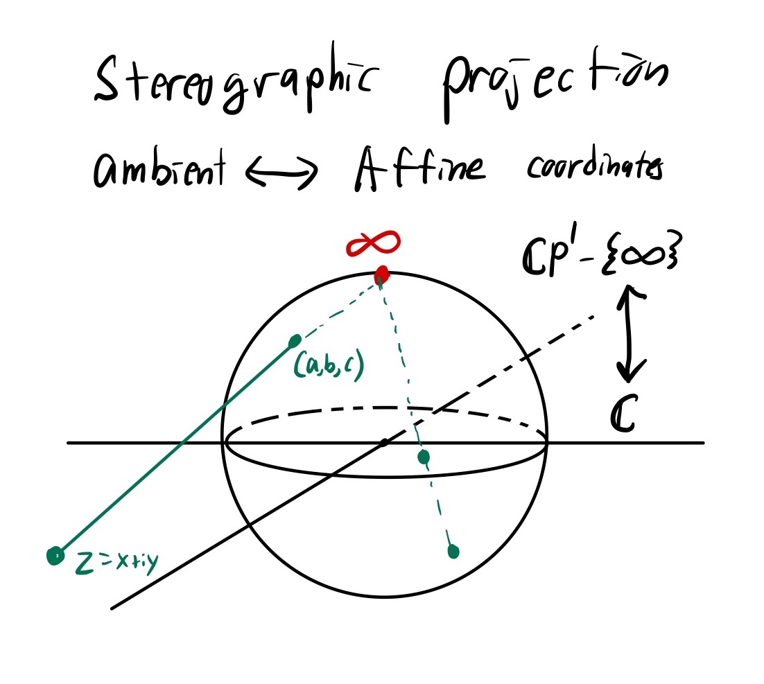
Stereographic projection

With the framework above, Stereographic projection is simply the change of coordinates from ambient / toric coordinates to affine coordinates. We will describe this in both sets of coordinates, but toric is much more convenient.

To sterographically project, sit $S^2$ as the unit circle placed around the origin of the plane $\mathbb{C}$. For every point $p\in S^2$ which is not the north pole (denoted by $\infty$), we draw a line from $\infty$ to $p$ and extend it until it intersects the plane. This gives a bijection between $S^2 - {\infty}$ and $\mathbb{C}$. Applying this projection to $\mathbb{C} P^1$, this gives the equivalence between the homogenous coordinates and affine coordinates.

The point $\infty$ in ambient coordinates is $(0,0,1)$. To project a point $(a,b,c) \in S^2$, we draw a parametrized line starting at $(0,0,1)$ and hitting $(a,b,c)$: $\gamma_t = t(a,b,c) + (1-t)(0,0,1)$ This intersects the plane $c=0$ when $tc + (1-t) = 0$, or $t = \frac{1}{1-c}$. Plugging this into $\gamma_t$, we get the conversion from ambient to affine coordinates.

Ambient $\implies$ Affine

\[(x,y) = \left(\frac{a}{1-c} , \frac{b}{1-c}\right) = (a\frac{K}{2}, b\frac{K}{2})\]

Where the Kahler potential is

\[K(a,b,c) = 1 + x^2 + y^2 = \frac{(1-c)^2 + a^2 + b^2}{(1-c)^2} = \frac{2}{1-c}\] \[\begin{align} \mathcal{D}_{(a,b,c) \to (x,y)} & = \begin{pmatrix} \frac{1}{1-c} & 0 & \frac{a}{(1-c)^2} \\ 0 & \frac{1}{1-c} & \frac{b}{(1-c)^2} \end{pmatrix} \\ & = \begin{pmatrix} \frac{K}{2} & 0 & a\frac{K^2}{4} \\ 0 & \frac{K}{2} & b\frac{K^2}{4} \end{pmatrix} \end{align}\]

Inverting the computation, or running the same technique in reverse, we get

Affine $\implies$ Ambient

\[(a,b,c) = \left(\frac{2x}{K(x,y)} , \frac{2y}{K(x,y)}, 1-\frac{2}{K(x,y)}\right)\]

where $K(x,y) = 1+x^2+y^2$. To compute the Jacobian, its helpful to coallate some computations:

$\partial _x K = 2x$, and $\partial _y K = 2y$
$\partial _x \frac{1}{K} =\frac{-2x}{K^2}$ We compute:

\[\begin{align} \mathcal{D}_{ (x,y) \to (a,b,c)} & = \begin{pmatrix} \frac{\partial a }{\partial x} & \frac{\partial a }{\partial y} \\ \frac{\partial b }{\partial x} & \frac{\partial b }{\partial y} \\ \frac{\partial c }{\partial x} & \frac{\partial c }{\partial y} \end{pmatrix} \\ & = \begin{pmatrix} \frac{2}{K} - \frac{4 x^2}{K^2} & - \frac{4 xy}{K^2} \\ - \frac{4 xy}{K^2} & \frac{2}{K} - \frac{4 y^2}{K^2} \\ -\frac{4x}{K} & -\frac{4y}{K} \end{pmatrix} \\ & = \begin{pmatrix} \frac{2}{K} - a^2& -ab \\ -ab & \frac{2}{K} - b^2\\ -2a & -2b \\ \end{pmatrix} \end{align}\]

I could find the Jacobian, but I don’t think its that kind of night.

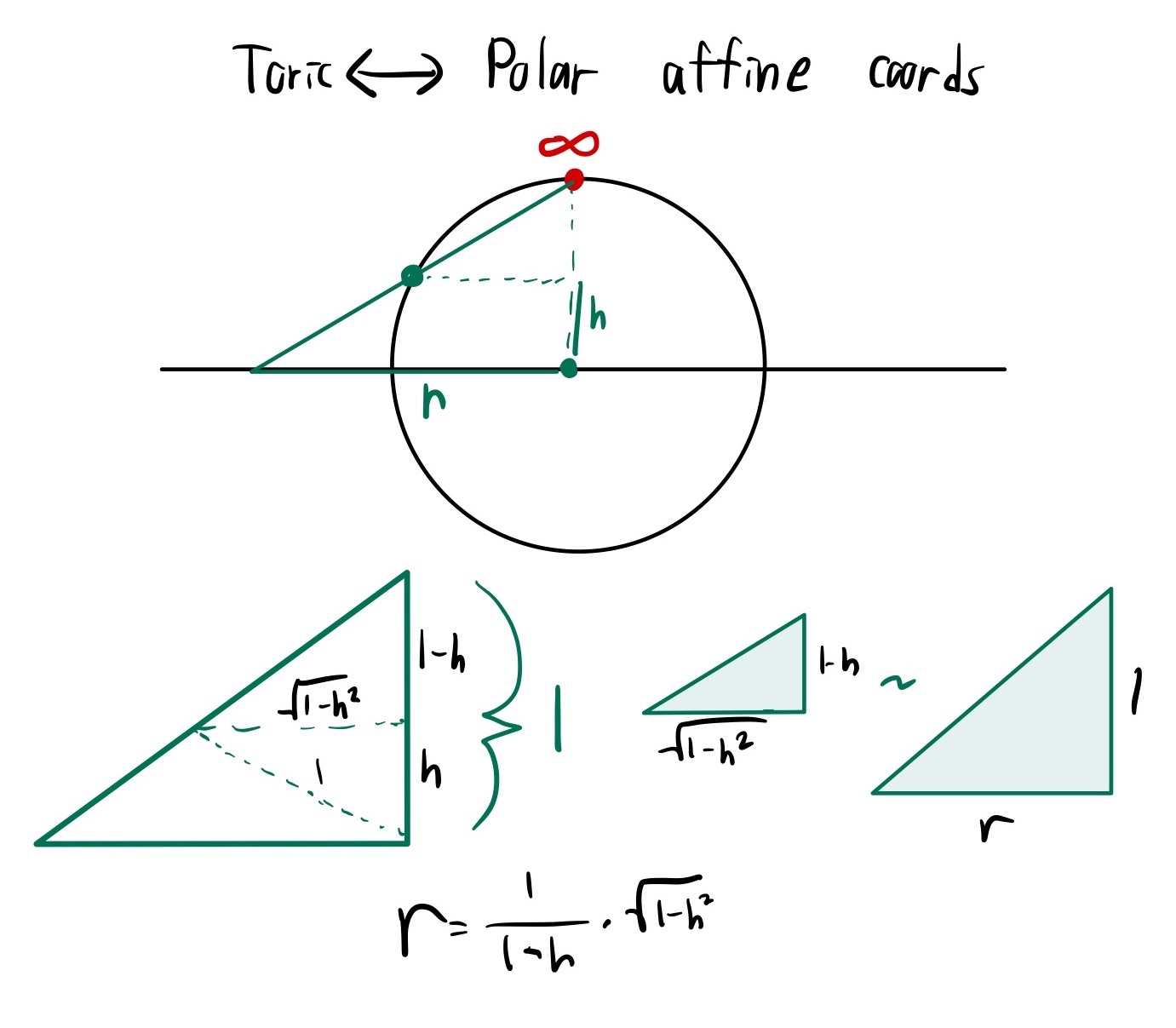
toric coordinates <–> polar affine coordinates

Toric $\iff$ Affine

\[\begin{align} (\theta,r) &= \left(\theta, \frac{\sqrt{1-h^2}}{1-h}\right) = \left(\theta, \sqrt{\frac{1+h}{1-h}}\right) \end{align}\]

The Kahler potential is $K = 1+r^2 = 1 + \frac{1+h}{1-h} = \frac{2}{1-h}$

\[\mathcal{D}_{(\theta,h) \to (\theta,r)} = \begin{pmatrix} \frac{\partial \theta }{\partial \theta} & \frac{\partial \theta }{\partial h} \\ \frac{\partial r }{\partial \theta} & \frac{\partial r }{\partial h} \end{pmatrix} = \begin{pmatrix} 1 & 0 \\ 0 & \frac{1}{(1-h)^2 \sqrt{\frac{1+h}{1-h}}} \end{pmatrix} = \begin{pmatrix} 1 & 0 \\ 0 & \frac{K^2}{4} \frac{1}{r} \end{pmatrix}\]

The angle stays the same after projecting, so to compute we only need to find the stereographically projected radius $r$ as a function of $h$. We can do this with some simple geometry, shown below. Everyone loves similar triangles.

Projective coordinates <–> Ambient coordinates

We can find the coordinate form of this stereographic projection by first sending $(a,b,c)$ to affine coordinates, then choosing a suitable lift to projective coordinates. Recall that we want $(x,y) = (\frac{a}{1-c},\frac{b}{1-c})$, meaning $z = \frac{a+ib}{1-c}$. One suitable map is $[Z_0:Z_1] = (1-c,a+ib)$The image in the affine coordinates $Z_1 / Z_0$ is exactly the steographic projection $(x,y)$.

Ambient $\iff$ Projective

\[[Z_0:Z_1] = (1-c,a+ib)\] \[\mathcal{D}_{(a,b,c)\to (Z_0,Z_1)} = \begin{pmatrix} 0 & 0 & -1 \\ 1 & i & 0\end{pmatrix}\]

We think of this coordinate map as $\mathbb{R}^3 \to \mathbb{C}^2$. When projected with to $\mathbb{C} P^1$, this gives the sterographic projection.

Metrics on $\mathbb{C} P^1$

Theorem

For $\mathbb{C} P^1$, the fubini-studi form in affine coordinates $z \in \mathbb{C}$ is

\[\omega_{FS} = \frac{i}{2}\frac{\mathrm{d} z \wedge \mathrm{d} \bar{z}}{(1+\vert z\vert ^2)^2}\]

Or, in real coodinates $z = x+iy$, denoting the Kahler potential by$K = 1+x^2 + y^2$,

\[\omega_{FS} = \frac{\mathrm{d} x \wedge \mathrm{d} y}{(1 + x^2 + y^2)^2} = \frac{\mathrm{d} x \wedge \mathrm{d} y}{K^2}\]

Proof

Apply the general formula for the fubini-Study form. In this case, there is only one index $i=j=1$. So, we get

\[\begin{align} \omega_{FS} &= \frac{i}{2} \frac{(1 + \vert z\vert ^2) \partial ta_{11} - \bar{z}_1 z_i}{(1+\vert z\vert ^2)^2} \mathrm{d} z \wedge \mathrm{d} \bar{z}\\ &= \frac{i}{2} \frac{(1 + \vert z\vert ^2) - \vert z\vert ^2}{(1+\vert z\vert ^2)^2} \mathrm{d} z \wedge \mathrm{d} \bar{z}\\ &= \boxed{\frac{i}{2} \frac{\mathrm{d} z \wedge \mathrm{d} \bar{z}}{(1+\vert z\vert ^2)^2}} \\ \end{align}\]

To turn this into real coordinates, we note $\vert z\vert ^2 = x^2 + y^2$. We just need to convert the forms. Use the computation:

\[\mathrm{d} z \wedge \mathrm{d} \bar{z} = (\mathrm{d} x + i \mathrm{d} y) \wedge (\mathrm{d} x - i \mathrm{d} y) = -i \mathrm{d} x \wedge \mathrm{d} y + i \mathrm{d} y \wedge \mathrm{d} x = -2i \mathrm{d} x \wedge \mathrm{d} y\]

Therefore $\frac{i}{2} \mathrm{d} z \wedge \mathrm{d} \bar{z} = \mathrm{d} x \wedge \mathrm{d} y$,. Plugging this in to the formula above, we get the real coordinates of the Fubini-Study metric.

Let us write $\omega_{FS}$ in the different coordinates.

Projective coordinates:

$\omega_{FS} = \frac{i}{2} \frac{\mathrm{d} Z_0 \wedge \mathrm{d} \bar{Z_0} + \mathrm{d} Z_1 \wedge \mathrm{d} \bar{Z}_1}{\vert Z\vert ^2} = \frac{i}{2} \frac{\mathrm{d} Z_0 \wedge \mathrm{d} \bar{Z_0} + \mathrm{d} Z_1 \wedge \mathrm{d} \bar{Z}_1}{K^2}$ This comes from the general result of the Fubini-Study form in projective spaces above.

Polar affine coordinates:

\[\omega_{FS} = \frac{1}{K^2} r \mathrm{d} r \wedge \mathrm{d} \theta = \frac{r}{(1+r^2)^2} \mathrm{d} r \wedge \mathrm{d} \theta\]

To prove this, we only used the standard radial volume form $\mathrm{d} x \mathrm{d} y = r \mathrm{d} r \mathrm{d} \theta$.

Toric coordinates: Looking at the rows of the Jacobian for Toric -> polar affine coordinates, we see that $\mathrm{d} \theta$ is preserved, and

\[\mathrm{d} r = \frac{K^2}{4} \frac{1}{r} \mathrm{d} h\]

Pulling back the Fubini-Study form for polar affine coordinates, the $K^2$ and $\frac{1}{r}$ cancel out, and we get

\[\omega_{FS} = \frac{1}{4} \mathrm{d} h \wedge \mathrm{d} \theta\]

This is why I introduced toric coordinates: They are the action-angle coordinates of $\mathbb{P}^1$, and it makes the symplectic structure very simple.

Ambient coordinates

The round metric on the sphere is defined in ambient coordinates by the 2-form

\[\omega_R = a \mathrm{d} b \wedge \mathrm{d} c + b \mathrm{d} c \wedge \mathrm{d} a + c \mathrm{d} a \wedge \mathrm{d} b\]

To show that how the Fubini-Study form plays with the round metric, we need to pull the round metric back from ambient coordinates to one of the 2D coordinate systems (What we tried before is to pull the 2D metric back to 3D and work there, which caused issues.)

To do this, I will use a map $\phi$ from toric coordinates to ambient coordinates (I could also do affine coordinates to ambient coordinates, but I haven’t yet computed that Jacobian.) We have the following pullbacks. We will continue to write the Coefficents in ambient coordinates, despite the forms living in toric coordinates, for ease of manipulation. Just remember that $a^2 + b^2 + c^2 = 1$.

From the Jacobian, we have the following formula for the pullbacks of forms from the ambient coordinates:

\[\begin{align} \phi^* \mathrm{d} a &= -b \mathrm{d} \theta - \frac{a c}{1-c^2} \mathrm{d} h\\ \phi^* \mathrm{d} b &= a \mathrm{d} \theta - \frac{b c}{1-c^2} \mathrm{d} h\\ \phi^* \mathrm{d} c &= \mathrm{d} h\\ \end{align}\]

We want to compute the pullback $\phi^* \omega_R$. The pullback will be some multiple of $\mathrm{d} \theta \wedge \mathrm{d} h$. That multiple is:

\[\begin{align} \frac{\phi^* \omega_R}{\mathrm{d} \theta \wedge \mathrm{d} h} &= c \begin{vmatrix}-b & -\frac{ac}{1-c^2} \\ a & -\frac{bc}{1-c^2}\end{vmatrix} + a \begin{vmatrix}a & -\frac{bc}{1-c^2} \\ 0 & 1\end{vmatrix} + b \begin{vmatrix}0 & 1 \\-b & -\frac{ac}{1-c^2} \end{vmatrix} \\ &= c\left(-(b^2+a^2) \frac{-c}{1-c^2}\right) + a ^2 + b^2 \\ &= c\left((1-c^2) \frac{c}{1-c^2}\right) + a ^2 + b^2 \\ &= c^2 + a ^2 + b^2\\ &= 1 \end{align}\]

I was stuck in “missing minus sign” purgatory for a while there :(. Be careful when you take derivatives, kids. Hence, we have proven:

Theorem: Relation between Fubini-Study and round metric

For $\mathbb{C} P^1 \cong S^2$, the Fubini-Study metric is 1/4 times the standard round metric for a sphere of radius 1. in particular, $\int_{S^2}\omega_{FS} = \pi$.

Since I have the mic, here is a nicer argument. From its projective description, the Kahler potential $\vert Z\vert ^2$ is invariant under $SU(2)$, thus $SU(2)$ must act by Kahler Isometries. This action descends to an action of the group $SO(3)$ on $S^2$ by rotations, meaning the Metric on $S^2$ must be symmetric. Therefore, it must be some scaling of the round metric. To find the scaling constant, we can find the area, by intergeatinrg $\omega_{FS}$ in affine coordinates over $\mathbb{C}$. This reduces to an explicitly solvable integral, whose value is $\pi$.

How not compute the fubini-study form

We derived the above by pulling back the round metric from $\mathbb{R}^3$ to $S^2$. We could imagine pulling back from $S^2$ to $\mathbb{R}^3$, and seeing what form you get. This won’t generally agree with the usual presentation of the round metric. Let’s investigate:

There is no well-defined pullback of the Fubini-Study form onto the ambient coordinates, because there are too many degrees of freedom. If we naively pull back $\omega_{FS}$ using any of the maps from $(a,b,c)$ to $S^2$, then we’ll get a form for all $(a,b,c)$, even those which don’t satisfy $a^2 + b^2 + c^2=1$. To satiate our curiosity, let’s see what this form can be.

Let’s start by pulling back from toric coordinates. Looking at the Jacobian, we have

\[\phi^* \mathrm{d} h = \mathrm{d} c \qquad \phi^* \mathrm{d} \theta = \frac{-b \mathrm{d} a + a \mathrm{d} b}{a^2 + b^2}\]

so the Fubini-Study form should be

\[\phi^*\omega_{FS} - \frac{1}{4} \left( \frac{-b}{a^2 + b^2} \mathrm{d} a \wedge \mathrm{d} c + \frac{a}{a^2 + b^2} \mathrm{d} b \wedge \mathrm{d} c\right)\]

Now let’s pull back from affine coordinates under stereographic projection. Looking at the Jacobian, we have

\[\phi^* \mathrm{d} x = \frac{K}{2} \mathrm{d} a + b\frac{K^2}{4} \mathrm{d} c \qquad \phi^* \mathrm{d} y = \frac{K}{2} \mathrm{d} b + a\frac{K^2}{4} \mathrm{d} c\]

So the pulled-back Fubini-Study form is

\[\begin{align} \phi^* \omega_{FS} &= \frac{1}{K^2} \phi^* \mathrm{d} x \wedge \phi^* \mathrm{d} y \\ &= \frac{1}{K^2}\left(\frac{K}{2} \mathrm{d} a + a\frac{K^2}{4} \mathrm{d} c \right)\wedge \left(\frac{K}{2} \mathrm{d} b + b\frac{K^2}{4} \mathrm{d} c \right) \\ &= \frac{1}{4} \left(\mathrm{d} a \wedge \mathrm{d} b + a \frac{K}{2} \mathrm{d} c \wedge \mathrm{d} b + b\frac{K}{2} \mathrm{d} a \wedge \mathrm{d} c\right) \end{align}\]

This does not equal the pulled back form above, even when $a^2 + b^2 + c^2 =1$!! This is possible because the two forms only need to agree on $T S^2$. We need to assume $a^2 + b^2 + c^2 = 1$, and that the vector we plug in lives in $T S^2$, i.e that it is perpendicular to $(a,b,c)$. Presumably these two forms agree on that subspace, but I’m too lazy to check.