Floer Equations with neural networks

Click and drag between highlighted orbits to view Floer cylinders

An interactive applet displaying numerical solutions of Floer’s equations. To define these equations, we first specify a function $H:\mathbb{C} \to \mathbb{R}$, which we will call the Hamiltonian. The Floer equations are a PDE describing maps from a cylinder $\mathbb{R} \times S^1$ (parametrized by $(s,t)$) to the complex plane $\mathbb{C}$. A map $u:\mathbb{R} \times S^1 \to \mathbb{C}$ satisfies the Floer equations when

We are interested in solutions to this equation (Called Floer cylinders) which limit to orbits of this Hamiltonian. That is, the limiting path $\lim_{s \to \pm \infty} u(s,t) = \gamma_{\pm}(t)$ is defined, and satisfies

A curve $\gamma$ satisfying this equation is called a Hamiltonian orbit. Each curve in the applet above is a 1-periodic Hamiltonian orbit. Clicking and dragging between two curves shows a Floer cylinder which limits to the first curve as $s \to -\infty$ and the second as $s\to -\infty$. I only display index 1 Floer cylinders, which are the solutions relevant for computing Hamiltonian Floer Homology

I solved the Floer equations numerically using a Physically Informed Neural Network (PINN) (See my methodology below). To my knowledge, these are the first numerical solutions to the Floer equations. After showing off an early gif of my Floer cylinder, I learned that Yuan Yao and James Rowan were also using PINNS to solve the related pseudoholomorphic curve equations! They just released a paper numerically finding compact pseudoholomorphic curves in compact manifolds¹. This blog post is perhaps a companion piece to their paper. James and Yuan have done real science, having fine-tuned their training regimen and compared PINNs to the ground truth or other numerical methods. I’m content with drawing pretty pictures. Many thanks to them for discussions and neural network help.

To make this post friendlier, I’ll start the basic framework of Symplectic geometry and PINNs. The last two sections of this post have more specifics about my numerics.

Background on Floer’s equations

Let me describe why we care about the floer equations.

The action functional

Symplectic geometry is the study of phase space of classical mechanics. Consider, for example, a particle attached to a spring in one dimension. The state of the particle is described by its position $x$ and momentum $p$, which we represent as a point on the plane $(x,p) \in \mathbb{R}^2$. This plane is phase space. The evolution of this particle is dictated by the total energy of the system, which is the sum of kinetic energy ($\frac{1}{2}p^2$) and potential energy (For a particle on a spring, $\frac{1}{2}x^2$). The total energy is a function on phase space called the Hamiltonian $H(x,p) = \frac{1}{2}(p^2 + x^2)$. The system evolves in phase space according to a vector field $X_H$ associated to the Hamiltonian, obtained by rotating the gradient by 90 degrees. This is clearest when we represent phase space as the complex plane $\mathbb{C}$ with $z = x+ ip$. Representing the gradient $\nabla H(z)$ as a complex number, our system flows along the vector field $X_H = i \nabla H$. For $H = x^2 +p^2 = \lvert z\rvert^2$, we get $X_H = iz$, which rotates phase space in a circle. ²

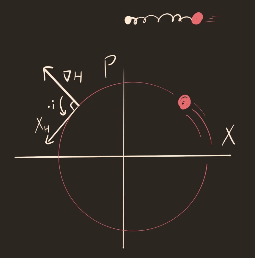
The motion of a particle on the spring (top) captured by a Hamiltonian vector field in phase space (bottom)

A core question in classical mechanics is, what are the periodic orbits of $X_H$ with period 1? To study this, we embed the periodic orbits in the space of all 1-periodic paths $\gamma : S^1 \to \mathbb{C}$. We call the space of $\gamma$ the loop space $\mathcal{L}(\mathbb{C})$, and note that $\gamma$ is an orbit of $X_H$ when $\dot{\gamma} = X_H$. Inspired by 100s of years of physics, we turn this into a variational problem. Construct the action functional $\mathcal{A}_H:\mathcal{L}(\mathbb{C}) \to \mathbb{R}$ whose critical points are exactly the 1-periodic orbits of $X_H$.

here $\text{Area}(\gamma)$ represents the signed area enclosed by $\gamma$, which is positive when $\gamma$ is counterclockwise.

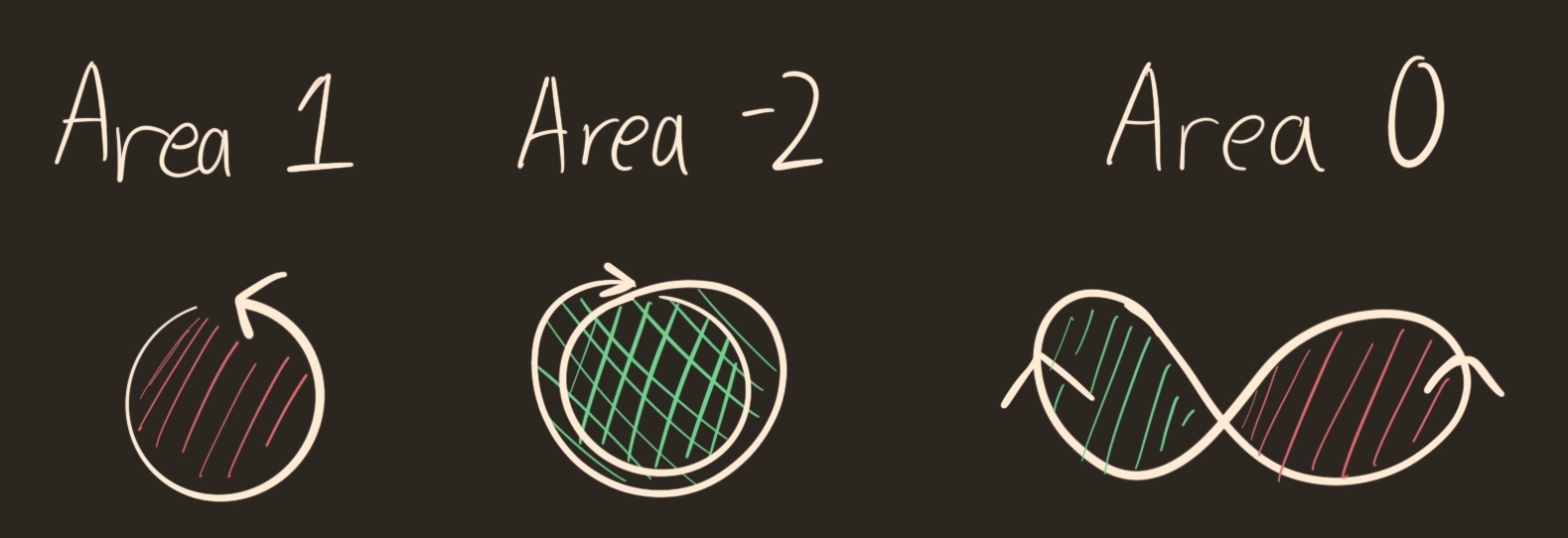
Examples of signed area, with my sign conventions

Gradient flow of the action functional

Floer’s idea was to count critical points of the action functional topologically. The key analogy comes from morse theory, which shows that the topology of a (finite dimensional) manifold forces functions to have a certain number of critical points. In the 60s, Arnold conjectured that counts of 1-periodic orbits satisfy the same bounds. Inspired by Witten’s work, Floer built an invariant out of critical points of $\mathcal{A}_H$, connected by flow lines of $-\nabla \mathcal{A}_H$.

Let’s take a step back. $\mathcal{A}_H$ is a function on the infinite dimensional loop space $\mathcal{L}(\mathbb{C})$, so a flow line is a path of loops $\gamma_s$.

A path of loops can be succinctly encoded as a map $u:\mathbb{R} \times S^1 \to \mathbb{C}$ from the cylinder into the complex plane, defined in coordinates by $u(s,t) = \gamma_s(t)$. This cylinder is a gradient flow line of action if it satisfies the Floer equations

We are looking for gradient flow lines connecting critical points, meaning the cylinder limits to Hamiltonian orbits

These Floer cylinders are very hard to find. Analytical, is impossible to solve Floer’s equations, owing to the nonlinearity in $\nabla H(u)$. Symplectic topologists have nonconstructive tools for proving the existence of solutions, but they rely on hard technical theorems and decades of development of the field. Numerically, they’re a huge pain. We can see the difficulty already when $H=0$. Here’s a solution to Floer’s equation which converges to a critical point:

Here’s a solution with initial condition perturbed by $10^{-6}$.

The solutions gets close to zero, then blows up. as an ODE, the Floer equations are unstable. We can see this explicitly when $H=0$. Then, the Floer equations $\partial_s u + i\partial_t u=0$ are linear, so can be solved via a Fourier transforms. If $a_n$ are the Fourier coefficients of $u(0,t)$, then the solution is

The only periodic orbits of $H=0$ (and hence the only critical points of action $\mathcal{A}_{0}$) are constant loops. If $u(+\infty,\cdot)$ is constant, then $a_{n>0} = 0$ but $a_{n\le0}$ is unrestricted. Conversely, if $u(-\infty,\cdot)$ is constant, then $a_{n<0} = 0$ and $a_{n\ge0}$ is unrestricted. In the language of dynamics, the stable and unstable manifolds of a critical point are both infinite dimensional. This property persists with arbitrary $H$. To find a floer cylinder, we need loop which converges in both positive and negative $s$. This lies on the intersection of two nearly complementary infinite dimensional manifolds. Finding this numerically is very delicate. The flow lines are like thin bridges stretching between mountains, and have to skydive onto them.

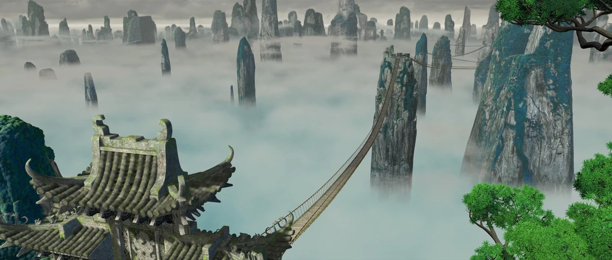
Numerically finding Floer cylinders

is like kung fu panda

I tried a bunch of random numerical techniques, with little success. What finally worked is a constrained optimization approach. I tie a string between the two mountain tops, and stretch it taught. That is, I apply an optimization algorithm to minimize the integrated error of floer’s equations. This is where the neural networks come in.

What is a physically informed neural network (PINN)?

Any numerical approach to solving partial differential equations (PDEs) has to contend with gulf between the finite memory of a computer and the infinite dimensionality of the space of functions. We always start by choosing a finite dimensional approximation of the space of functions. Here are some classic choices:

• Define a function as a set of values on a grid (finite element method).
• Define a function as a sum of Fourier modes (spectral methods). All of these are Linear representations, approximating a function as a sum of basis functions.³ A PINN opts for a Nonlinear representation of functions, as the output of a neural network. Here’s the structure of a neural network:

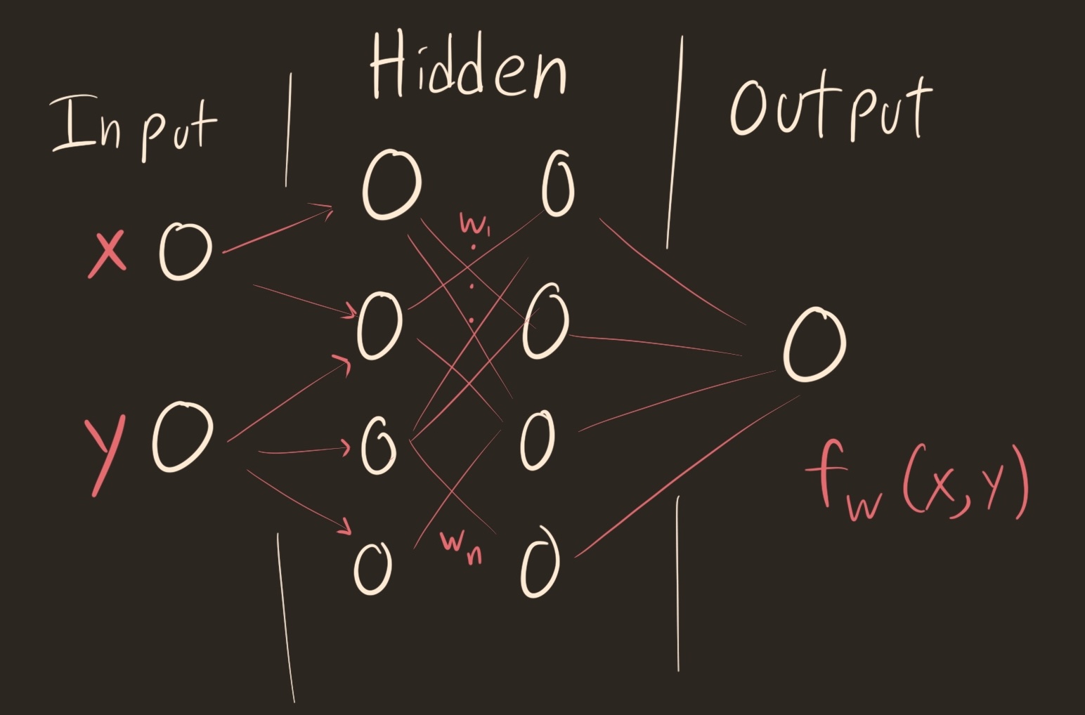
Internal structure of a neural network. Each line connecting two nodes is assigned a weight $w$. The collection of these weights determines a function $f_w$ from the input nodes (here, $x,y$) to the output node.

A neural network defines a function from the input layers to the output layer. Between each layer, the network takes the vector of values in the first layer, applies a matrix, then hits each entry of the resulting vector with a simple nonlinear function. I used tanh.

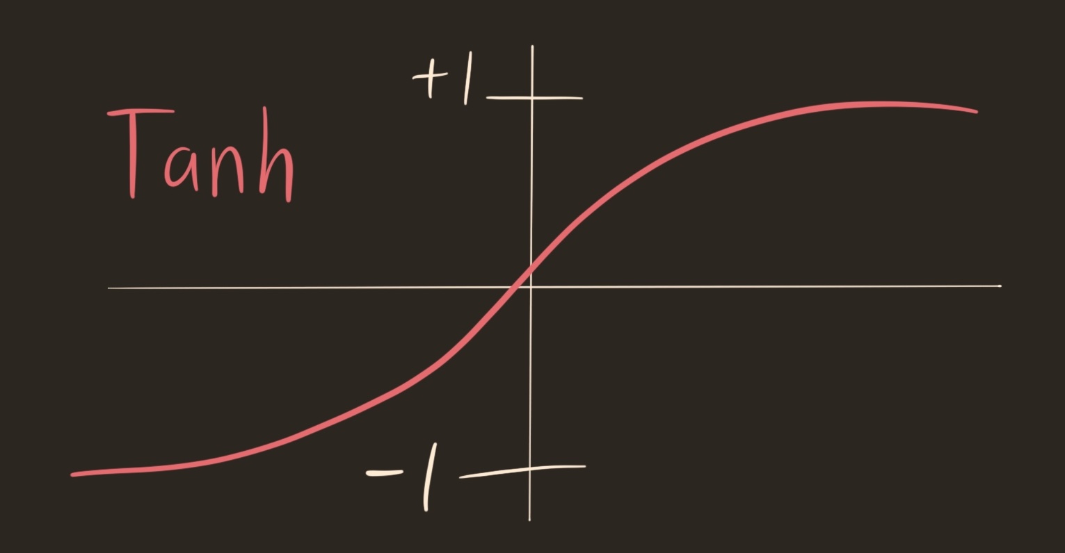
Apply this operation for each layer, then take one final linear combination to get the output value. You can approximate any function with a neural network. The resulting function is cheap to evaluate, and parametrized nonlinearly by the entries of the matrix. Let $f_w$ denote the function defined by weights $w$. The process of finding weights $w$ to make $f_w$ do what you want is called training the network. We first encode the behavior in some loss functional to be minimized $\mathcal{L}(f_w)$, then we optimize with respect to $w$ in one way or another.

How do we train $f_w$ to solve the PDE $\mathcal{F}(f_w)=0$? Set the loss function to equal the PDE itself!

This is the core insight of PINNs. Here’s some clever implementation details. he standard technique is to first apply a stochastic gradient descent algorithm to get us near the minimum, followed by quasi-newton’s method to polish things off. Both of these require knowing the derivative of $f_w$ with respect to the weights $w$. Since we are in a large dimensional space, finite differences wouldn’t work very well. Symbolic derivatives also wouldn’t work, because of the nonlinearities. Luckily, there’s a middle ground, called automatic differentiation.

In your computer, every function is realized as combinations of floating point operations of plus, times, minus, divide. The overall derivative could in principle be computed using a heroic sequence of chain rules. We can compute this chain rule one step at a time. When evaluating the network, we simultaneously keep track of the derivative with respect to the weights $w$, updating with every floating point operation. With little overhead, every evaluation comes bundled with the partial derivatives with respect to every variable. Since we’re computing all these derivatives already, evaluating the PDE at a point $\mathcal{F}(f_w)(x)$ is extremely convenient. To compute the overall loss, evaluate the neural network $f_w$ at $\sim3000$ points, compute the PDE loss at that point $\lvert \mathcal{F}(f_w)(x)\rvert^2$, and average.

All these details are fortunately hidden from the end user (me). Simply install pytorch, define your loss function, and choose your favorite optimizer. Unfortunately, it’s not plug and play. I had to chose a lot of parameters, and tune them to get the PINN to actually converge.

PINN methodology

Bounding the domain

In order to represent the domain $\mathbb{R}\times S^1$ numerically, I compactified the $s\in \mathbb{R}$ coordinate into $\sigma \in [-1,1]$:

A floer cylinder is represented as a map $u:[-1,1]_\sigma \times [0,2 \pi]_t \to \mathbb{C}$, with periodic boundary conditions in $t$ and Dirichlet boundary conditions in $\sigma$

As input to the PINN, I define the Hamiltonian and two parametrized 1-periodic Hamiltonian orbits $\gamma_{\pm}$. To ensure the boundary conditions are satisfied, I train my PINN to find a solution to the Floer equations relative to a baseline. Define the linear interpolation of the boundary conditions

By exploiting the vector space structure of $\mathbb{C}$, every cylinder can be parametrized as $u+\bar{u}$. If $u_w$ is the trained neural network, then I construct the function $\bar{u } + (1-\sigma^2) u_w$. The overall loss is

With the $(1-\sigma^2)$ cutoff, any smooth $t$-periodic function $u_w$ yields a cylinder with the correct asymptotic behavior. This architecture makes the boundary conditions automatic.

Restricting myself to time-independent Hamiltonians makes finding their periodic orbits easy. This introduces the subtlety that critical points of the action functional are almost always degenerate. Indeed, if $\gamma(t)$ is a Hamiltonian orbit of $X_H$, so too is $\gamma(t+ t_0)$. If $\gamma$ is not constant, then it comes with a circle worth of critical points. The standard resolution to this is to add a small, time-dependent perturbation to split the circle of critical points into only 2 critical points. I opted not to do this, because these sorts of shallow-sloped valleys are famously hard for optimizers. Instead, I searched for Floer cylinders in the unperturbed problem.

The unperturbed problem has an $S^1$ worth of cylinders, corresponding to reparametrization $u(s,t) \mapsto u(s,t+t_0)$. Therefore, there is always a cylinder satisfying $\lim_{s\to -\infty} u(s,t) = \gamma_{-}(t)$ for any parametrization of $\gamma_-(t)$. This nails down the parametrization of $\gamma_+(t)$. Therefore, we seek solutions $u$ with

where perhaps only one value of $t_0$ has a solution. I included $t_0$ as one of the learning parameters inside my stochastic optimization.

Fourier features

For my first layer, I did not input two nodes $\sigma,t$. Instead, I precomputed the first few Fourier modes of $\sigma$ and $t$, and fed those in. I made sure to use Fourier modes satisfying my desired boundary conditions. The functions I feed in are products of factors for $t$ and $\sigma$:

where $(k_\sigma,k_t)$ lies in a circle of specified radius. These are called Fourier features in the PINN literature. These achieve two goals. First, since every input is periodic in $t$, the resulting network will automatically satisfy periodic boundary conditions in $t$.

Second, the higher Fourier modes make the PINN more effective. When $H=0$, the remaining linear PDE is diagonalized by Fourier modes. So, if we give all the Fourier modes ahead of time, the PINN has to only learn a linear function. Turning on the perturbing function $H$, we expect that feeding the network the Fourier mode will shortcut the approximation process. PINNs tend to have bias towards smooth functions whose Fourier transform lives close to zero. Feeding in the higher Fourier modes mitigates that, and allows the PINN to learn sharper features. (my models performed ~1 order of magnitude better when including higher Fourier modes). For more details and best practices, see An Expert’s Guide to Training Physics-informed Neural Networks. The effectiveness of Fourier features for learning J-holomorphic curves is examined in James and Yuan’s paper¹. They point out that the high Fourier features are necessary for seeing bubbling, where the derivative of a $J$-holomorphic curve concentrates in a single point. This is a blessing because bubbling is an important $J$-curve phenomena, but a curse because it gives the PINN an easy local way to fail to converge. We are forced to impose some sort of smoothness in our loss function.

Training methodology

Here are the stats for my network:

• 2 hidden layers
• each hidden layer is 100 wide
• Fourier feature radius 5 (about 60 in total)
• tanh activation function

To train my network, I started with ADAM (a stochastic gradient descent algorithm) for 1500 epochs, followed by 30 steps of L-BFGS (A version of newtons method). L-BFGS is very powerful, but requires computing the loss at a fixed set of points and is susceptible to overfitting. Following James and Yuan ¹, I chose a uniform grid in $\sigma ,t$ spaced denser than my Fourier features. (Importantly, a uniform sampling in $s,t$ didn’t work very well). I didn’t do any fancy learning rate scheduling like James and Yuan. Because I cheaped out on nodes and training epochs, I got kinda crummy convergence. I measure the error by the pointwise size of $\lvert\mathcal{F}(u)\rvert^2$. For my converged curves, my maximal error was around $0.01 - 0.1$, and the average error about 5x less. Compared to James and Yuan, who consistently got mean errors of less than $10^{-5}$, I have a lot of room for improvement.⁴

Here’s a typical example of successful training. On the left panel, I plot a mesh of the Floer cylinder in the complex plane. On the right, I plot the pointwise error of the floer equations. Watch the error decrease as the training progresses.

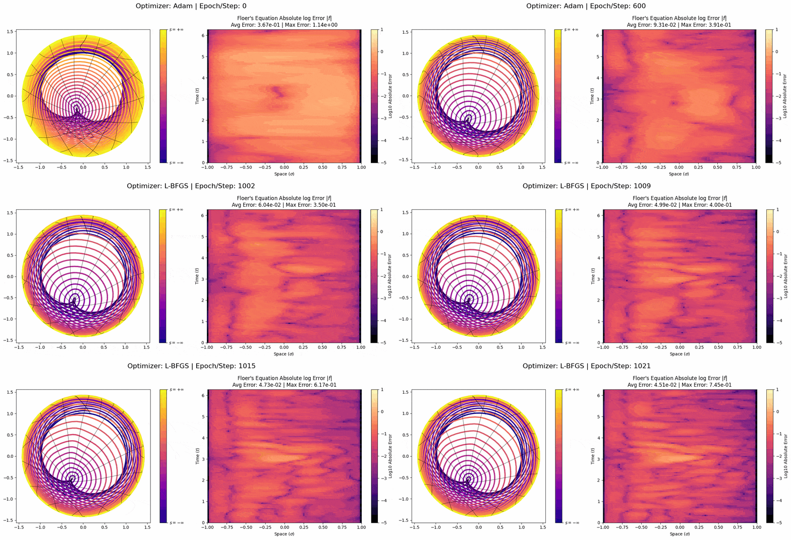
Training a successful curve, with Hamiltonian $H(z) = |z|^4$. This was from before adding Fourier features in $\sigma$, which is why the error in the right panel is horizontally banded

And here’s the same example boundary conditions with the input and output swapped (No floer cylinder can exist here, because the index is wrong). You see how the process does not converge (as it shouldn’t, the index is wrong). Usually, when things fail to converge, L-BFGS forces the error to be large in concentrated region.

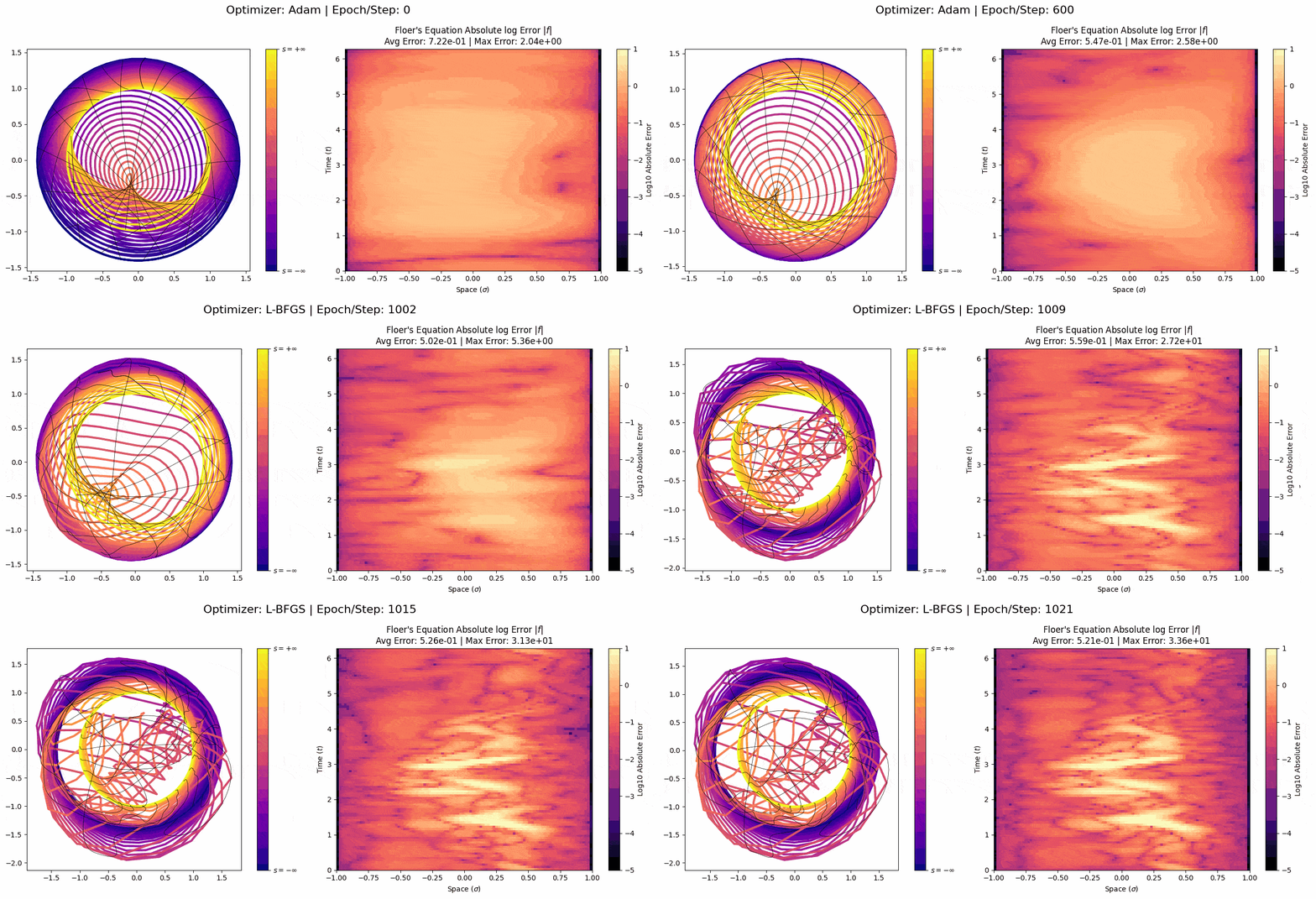
unsuccessful training of a floer cylinder. Train Floer cylinders which don't exist often leads to the flesh vortex on the right.

Numerical Floer Homology

Now that we can find Floer cylinders numerically, we try our hand at computing some invariants. For any Hamiltonian on the plane, we can associate the Morse homology of the action functional on loop space. This homology theory has underlying chain complex is generated by critical points of the action (i.e 1-periodic Hamiltonian orbits). Its differential counts one-dimensional moduli spaces of flow lines connecting the critical points (i.e index 1 Floer cylinders). The homology of this complex is called the Hamiltonian floer homology $HF^*(M,H)$ on a symplectic manifold $M$ with Hamiltonian $H$. From Floer and onwards, we know quite a lot this differential and its homology.

• Every 1-periodic orbit $\gamma$ has its Conley-Zehnder index, $\mu_{cz}(\gamma)$. See Audin-Damian for a definition. When $M \cong \mathbb{R}^2$, the Conley-Zehnder index is canonical and single-valued.
• The differential squares to zero, meaning we actually have a chain complex. The differential decreases the Conley-Zehnder index by 1.
• The homology of this chain complex is isomorphic to the reduced homology of the underlying manifold, so $HF^\ast(M,H) \cong H^\ast(M)$. For any Hamiltonian on $\mathbb{R}^2$, the Hamiltonian Floer homology is trivial. Even though the homology doesn’t tell us about the Hamiltonian, we can extract useful invariants of the Hamiltonian from the chain complex itself. (For instance spectral invariants or more ambitiously the full persistence barcode)

We dream of an oracle that takes in a Hamiltonian and computes this chain complex for us. My Applet is far from that. All it can do is pick Floer cylinder out of the soup with a leaky spoon. If the PINN fails to find a Floer cylinder, there may truly be none, or the training might have failed for any multitude of reasons. A converging PINN is pretty good evidence for a Floer cylinder, but it knows nothing about the number of cylinders or their relative orientation. But perhaps this morsel, combined with all the properties outlined above, is enough to nail down the complex.

The resting place of this project is a program where you type in a Hamiltonian, and it automatically finds all the periodic orbits and checks for all index 1 Floer cylinders. Then, you can upload your data into the explorer above and play. This almost exists. For now, I feel content to go through a few examples. You can play with these examples by selecting the corresponding choice from the dropdown above.

A Quartic Hamiltonian

\(H(x,y) = (x^2+y^2)^2\)

Consider the Hamiltonian above. The level sets of $H$ are all circles. The brave among you could compute the period of the hamiltonian vector field as a function of the level. I’ll rely on my computer. Here’s a graph: I put the period on the $x$-axis so that its shape emulates the profile of $H(z)$. (note that my “frequency” is $2\pi/T$ where $T$ is the period of the hamiltonian orbit)

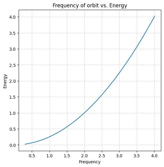
Graph of frequency $2 \pi/T$ versus level of the level set.

(note that I’ve added an extra $2 \pi$ factor everywhere. Qualitatively, it makes no difference.) Explicitly, $X_H$ has a 1-periodic orbit at level $2\sqrt{k}$ which wraps around $k$ times. Call this orbit $\gamma_k$. Remember the subtlety that due to reparamertizction, $\gamma_k$ is actually a degenerate circle of 1-periodic orbits. Apply a small time-varying perturbation, and split this circle of orbits into two orbits. Call the local minimum of the circle the elliptic orbit $\gamma_k^e$ and the local maximum the hyperbolic orbit $\gamma_{k}^h$. Computing the Conley-Zehnder index, we get

Finally the constant loop $\gamma_0(t)=0$ does not split, and has Conley-Zehnder index $\mu_{CZ}(\gamma_0) = 0$. All together, we have exactly one orbit of each nonpositive index. Let’s draw these generators on our graph. They occur where the graph intersects a vertical line $\text{frequency} = k$, and all intersections but the critical point split into two.

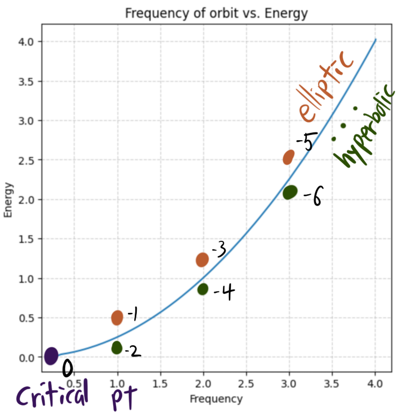
Generators of Hamiltonian Floer homology with $H(z) = \lvert z\rvert^4$.

The two orbits $\gamma_k^h$ and $\gamma_k^e$ arose from perturbing a circle of critical points. Morse-Bott yoga suggests that the morse flow lines of the circle persist as gradient flow lines of the action functional. That is, these two (slightly different) orbits are connected by a Floer cylinder rotating the parametrization of the loop by $\pi$. In fact, there are two flow lines, moving each direction around the circle. In fact in fact, these two flow lines have opposite orientation and thus cancel each-other out. We safely ignore the contribution of flow lines between pairs of previously degenerate orbits.

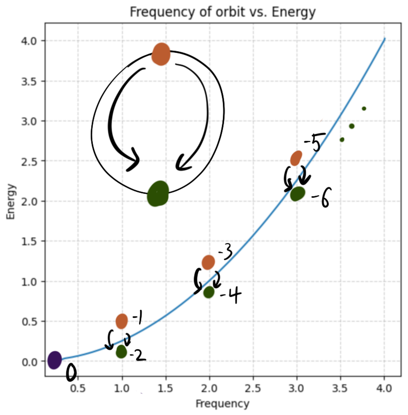
Coming from the morse flow lines of a circle (top left), we obtain double arrows between every pair of 1-periodic perturbed orbits, which cancel one another out.

We are left with a single generator in every index, and no differential connecting $-2k+1$ to $-2k$. For the overall homology to vanish, we must kill every generator. The only way to do this is to add Floer cylinders of frequency $k$ to the elliptic orbit of frequency $k+1$. Therefore, our chain complex looks like this:

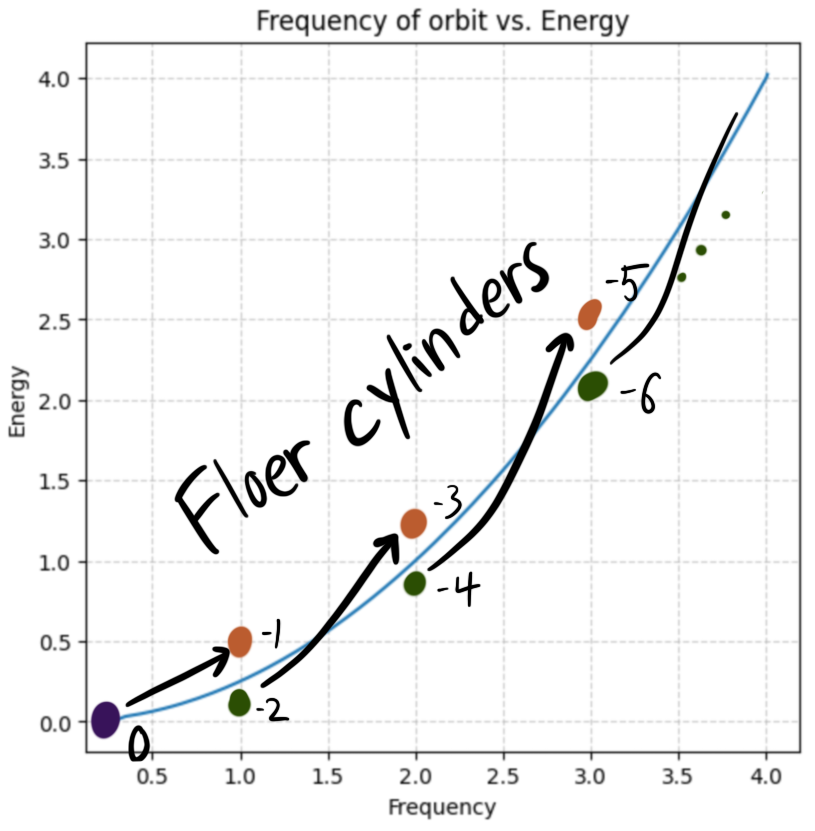
To ensure zero homology, we pair each generator with a friend

This is a non-constructive proof of the existence of Floer cylinders (most methods in symplectic geometry are no-constructive.) Collapsing back to the unperturbed hamiltonian, each periodic orbit needs one Floer cylinder attaching to the next largest orbit. With PINNs, we can finally construct them! You can see what Floer cylinders look like above. Here’s an animation of the $s=\text{const}$ slices of the Floer cylinder, as $s$ sweeps from $-\infty$ to $\infty$.

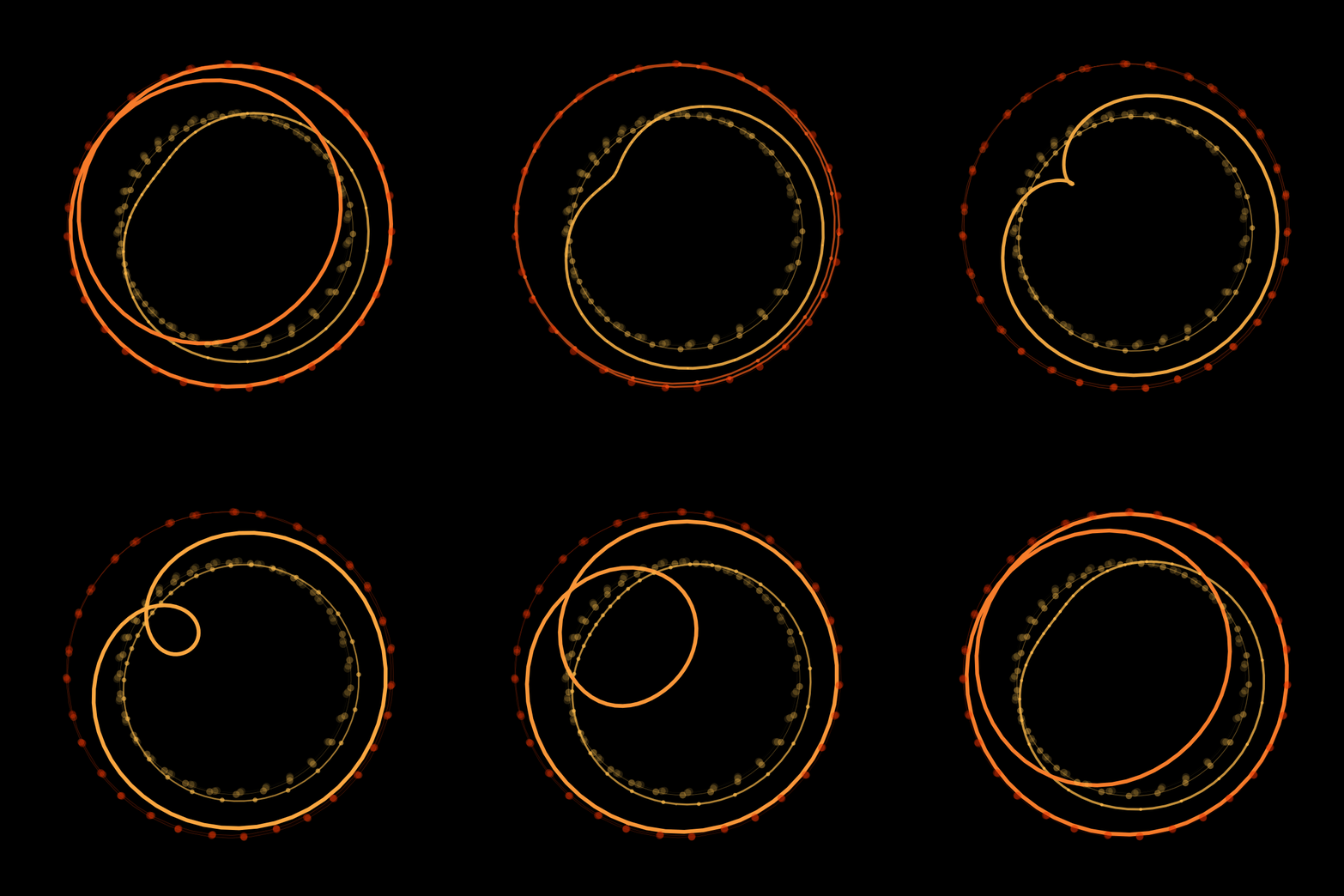
A Floer Cylinder

Note that I never did a perturbation to make things nondegenerate. Instead, I just searched for Floer cylinders connecting the two degenerate critical loci. So, I don’t know if the Floer cylinder connected to the elliptic or hyperbolic orbit, and don’t know the index of the resulting Floer cylinder. This is why in the info-box below the applet gives pairs of numbers.

Ive also included a couple more exotic hamiltonians (assessable via dropdown), along with every Floer cylinder I could find. Check the box “show non-converged floer cylinders” to see some classes of floer cylinders I could not find (I don’t know If i should be able to find any…) Play around with it!

Extensions

With this framework for learning Floer cylinders, I can finally try to make all these pictures of pseudoholomorphic curves and Floer cylinders I’ve always wanted. Here a wishlist of daydreams of mine, which are looking more tangible than ever. I’ve ordered these by the amount I would need to change the neural network architecture.

• Floer theory for Time-dependent Hamiltonians in the plane. In principle the PINN architecture wouldn’t need any modifications. The trouble is we can no longer easily enumerate the 1-periodic orbits. But if we numerically find some fixed points of the time 1 flow, then we can look for floer cylinders. The non-degeneracy might make it easier to train.
• Hamiltonian floer theory on toric manifolds. This was my original motivation. If we restrict to hamiltonians which are formed by composing the moment map with a smooth function, then we can once again explicitly describe the 1-periodic orbits. For example, the chain complex of the norm squared of the moment map has real applications. I would love to see the floer cylinders projected along the moment map, like I did with holomorphic curves here. Since Toric manifolds are quotients of vector spaces, it’s not too far off from the current framework. Alas, I haven’t managed to make any floer cylinders converge.
• Cylindrical contact homology and Birkhoff sections: finite energy J-holomorphic cylinders in the symplectization of contact manifolds limit to Reeb orbits. The projection of these to the three manifold gives surfaces connecting two Reeb orbits, which intersect every other orbit. These are called Birkhoff sections, and they are a very powerful dynamical tool for reducing Reeb dynamics to two dimensional surface dynamics. I’d love to see what the ones coming from $J$-curves look like. Also, similarly to hamiltonian floer homology, contact 3-manifolds have an invariant called cylindrical contact homology (CCH), which counts these holomorphic cylinders. Perhaps PINNs could numerically approach the CCH chain complex.
• Lagrangian floer homology: Cut open the cylinder to a strip, and demand the boundary of the strip lies on a Lagrangian submanifold. Asymptotically, these Floer strips limit to hamiltonian orbits starting and ending on the Lagrangian. For very small hamiltonians, the floer cylinders are known to limit to morse flow trees of the hamiltonian restricted to the Lagrangian.⁵ This is supposed to look like the convergence of an Amoeba to its topicalization. I’d love to see this in action.