Moduli stack of genus 3 curves
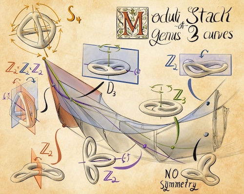
Drawing of a subset of the moduli stack of genus three curves, showing how how the loci of points in the stack with certain automorphism groups might interact. As we move from the top left to the bottom right, we go from more symmetric to less symmetric curves. Each symmetry has its own locus, drawn in its own color with representative curves drawn alongside. From the top, we have:
- $S_4$ tetrahedral symmetry, drawn in yellow
- $\mathbb{Z}_3$ rotational symmetry, drawn in green.
- $\mathbb{Z}_2$ reflection symmetry, drawn in orange.
- another $\mathbb{Z}_2$ reflection symmetry, drawn in blue.
- $\mathbb{Z}_2$ rotational symmetry, drawn in purple.
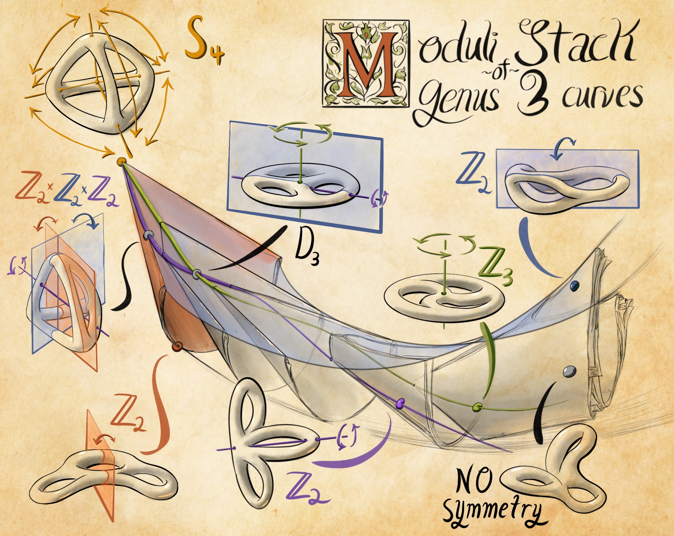
Fold your own moduli space
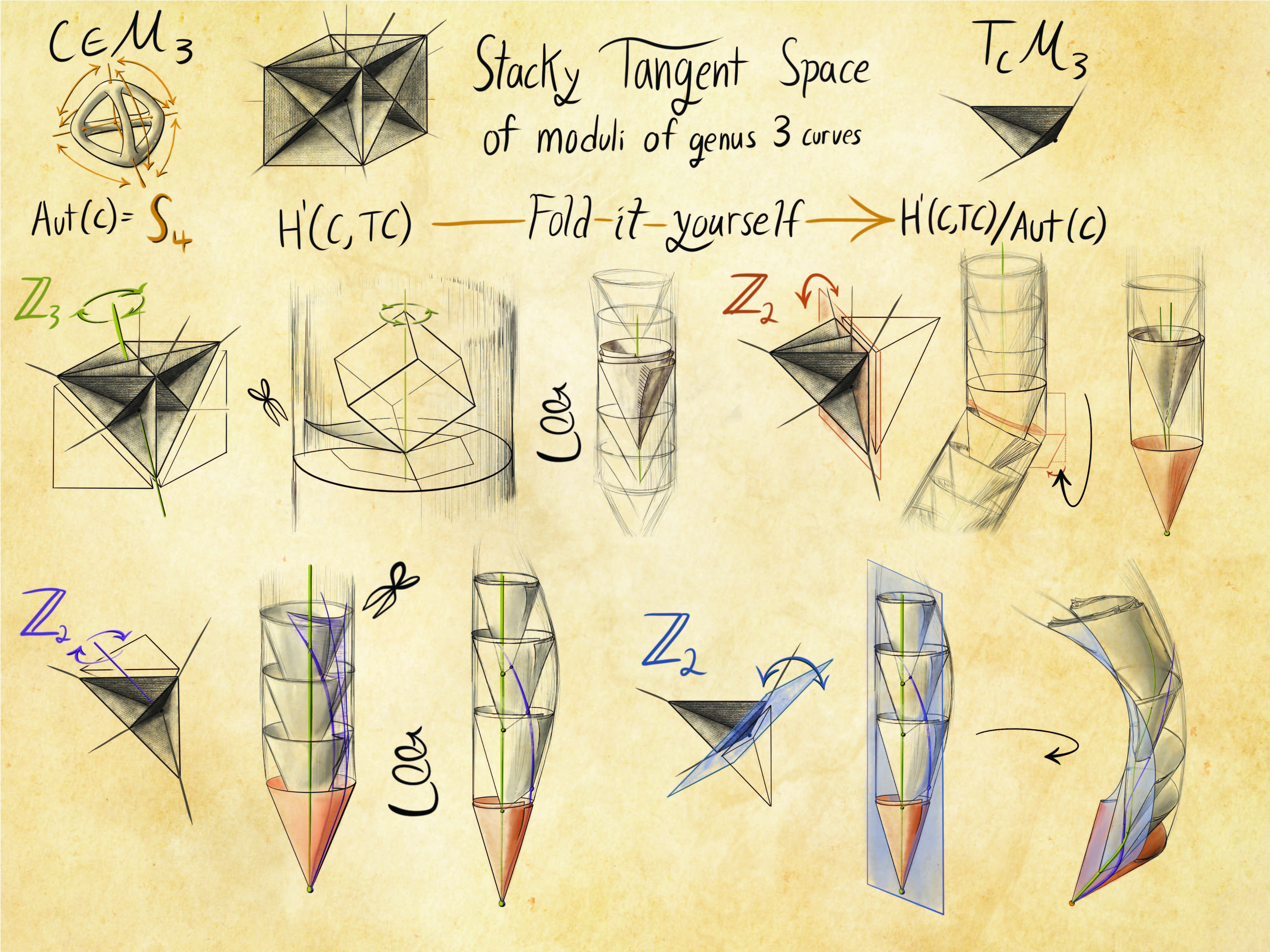
A stack is like an origami manifold. If the stack is Delinge-Mumford, then it is constructed by folding up a scheme by finite group actions. This figure shows the process of folding up a stack from an ordinary manifold. In this case, we want to understand the moduli space near a curve with especially high symmetry (in this case, $S_4$). Through a process of cuts, folds, and rolls, we obtain a folded up final space. The cube pictures show ths fundamental domain, restricting after each step. In the end, we are left with a fundamental domain which is $1/24^\text{th}$ the size of the original cube.
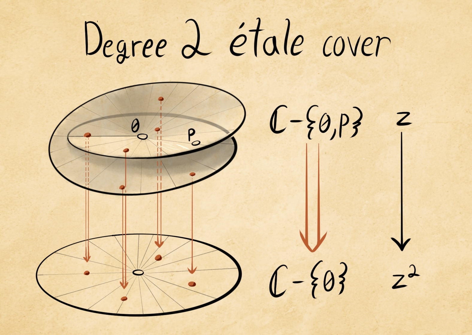
Etale covering
Example of an etale covering. This is a locally finite covering, but the number of sheets need not be constant. This could be due to a branch point, or a point missing from one of the sheets.
A quotient stack, and GIT quotient
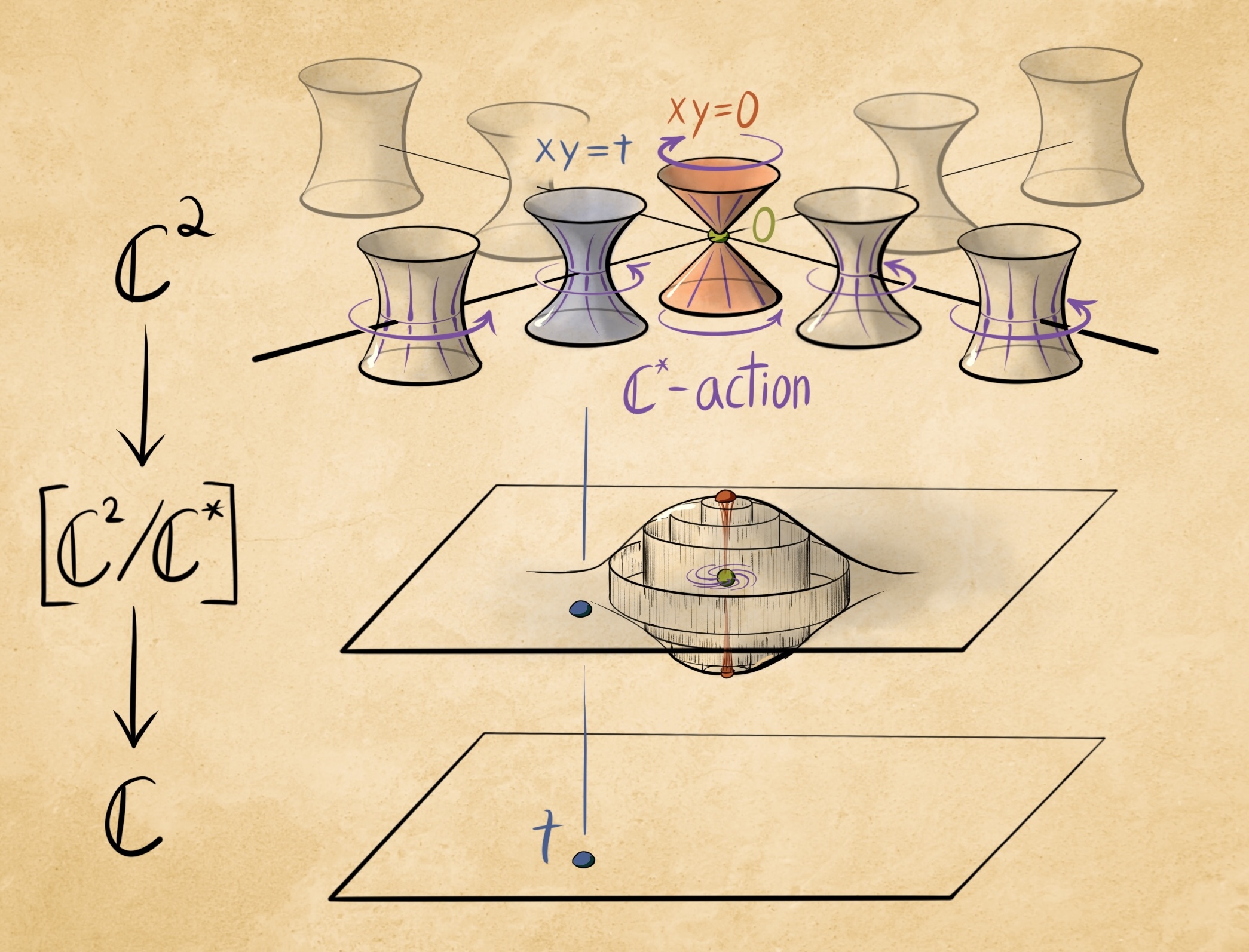
A picture of the action of $\mathbb{C}^\ast$ acting on $\mathbb{C}^2$ by multiplying each coordinate. That is, $\lambda \cdot (x,y) = (\lambda x, \lambda y)$ The orbits look like all look like complex hyperbolas, except for the central degenerate hyperbola. This has three components: The x-axis $\{y=0\}$, the y-axis $\{x=0\}$, and 0.
Passing to the quotient stack, the nondegenerate orbits are described by a single complex parameter $xy=t$, so the space of orbits looks like $\mathbb{C}^\ast$. Every neighborhood of the x-axis or the y-axis intersect one another, so the quotient space is non-hausdorff. It looks like a complex line with two origins. This is drawn in the middle layer by identifying the top and bottom layer of the raviolo. There is one extra point, corresponding to 0. This is in the closure of both the x-axis and the y-axis. This point is "stacky", meaning the associated orbit has nontrivial automorphism group (in this case, $\mathbb{C}^\ast$). This is represented by the little galaxy around the central point.
Finally, the bottom layer shows the GIT quotient $\mathbb{C}^2 // \mathbb{C}^\ast$. This is an honest hausdorf affine space. the three orbits of the x-axis, y-axis, and 0 are all identified. The resulting space is isomorphic to $\mathbb{C}$.
A nontrivial family
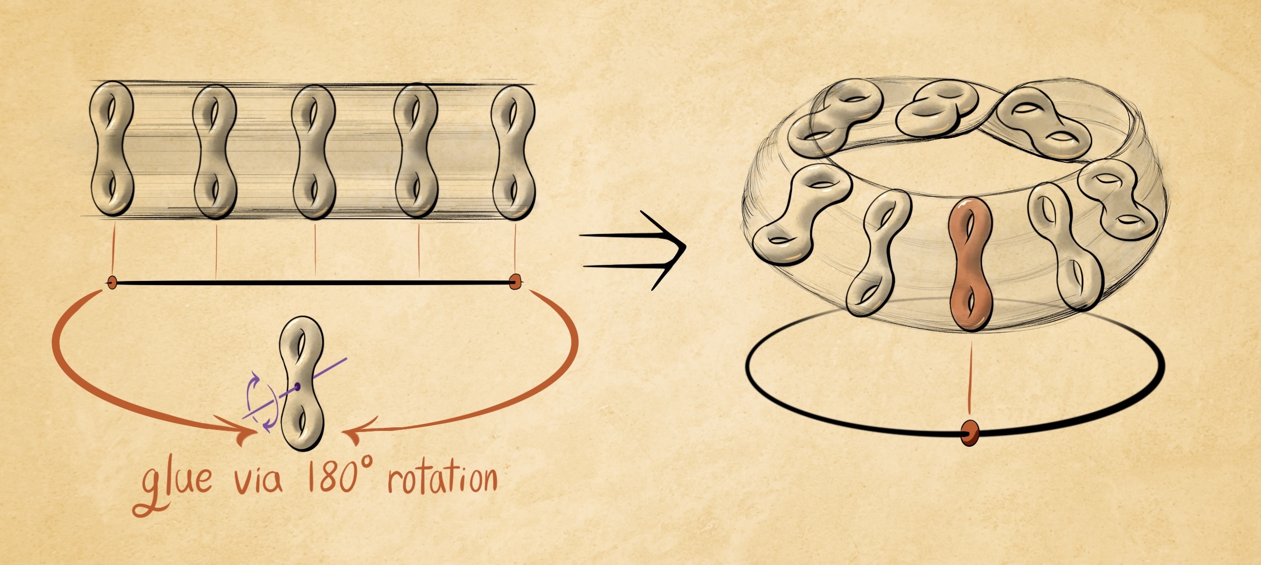
This image shows a nontrivial family of curves, with every curve in the family isomorphic. This is achieved by taking the mapping torus of an automorphism of the curve (in this case, a 180 degree rotation). The existence of such examples shows that the moduli problem of algebraic curves cannot be classified by maps into a scheme. Instead, we need a stack.
covers of nodal curves
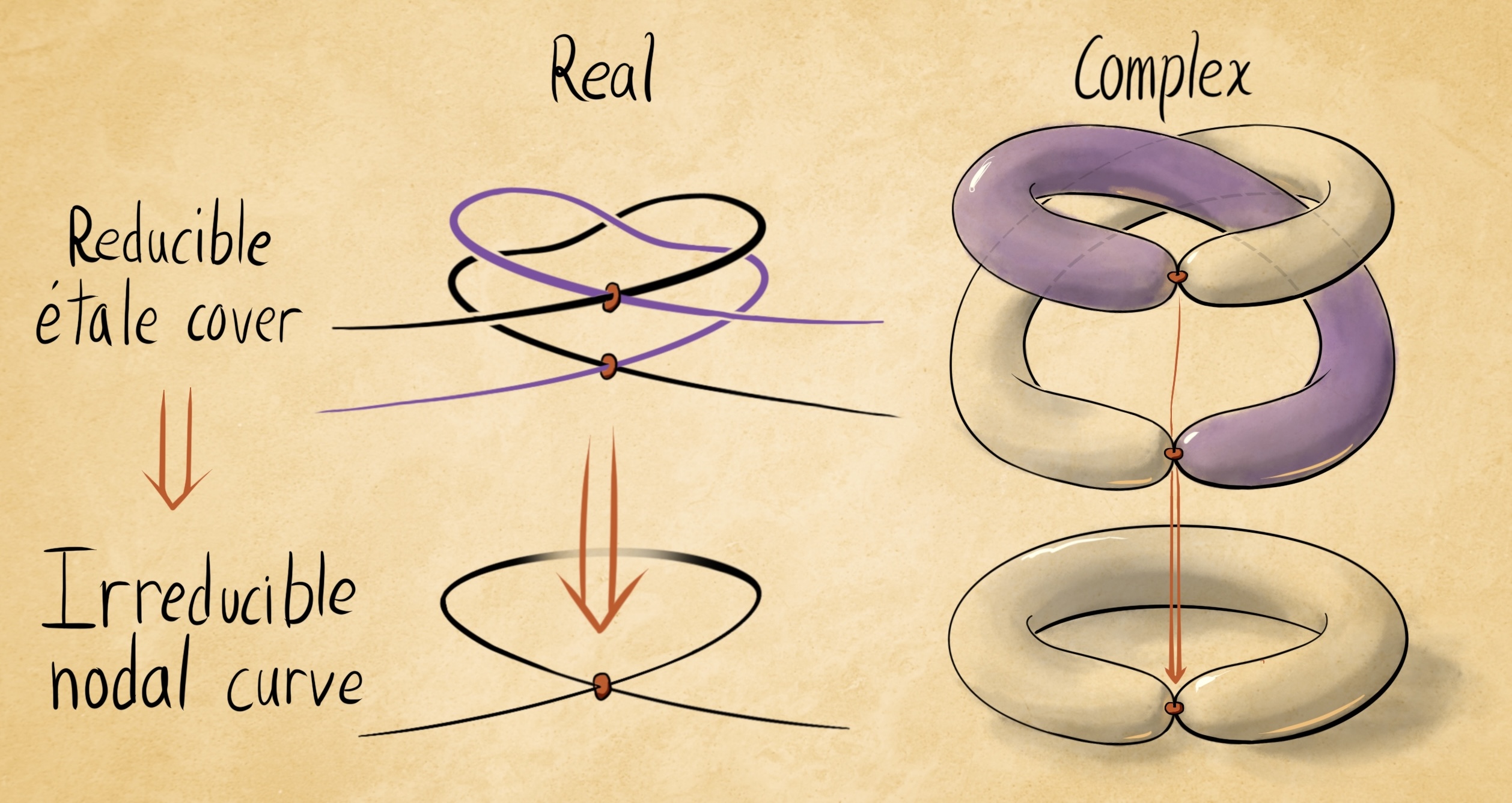
An irriducible nodal curve can be made reducible by taking an Etale cover. On the left is the picture over $\mathbb{R}$, on the right the picture over $\mathbb{C}$.
Moving through the moduli space
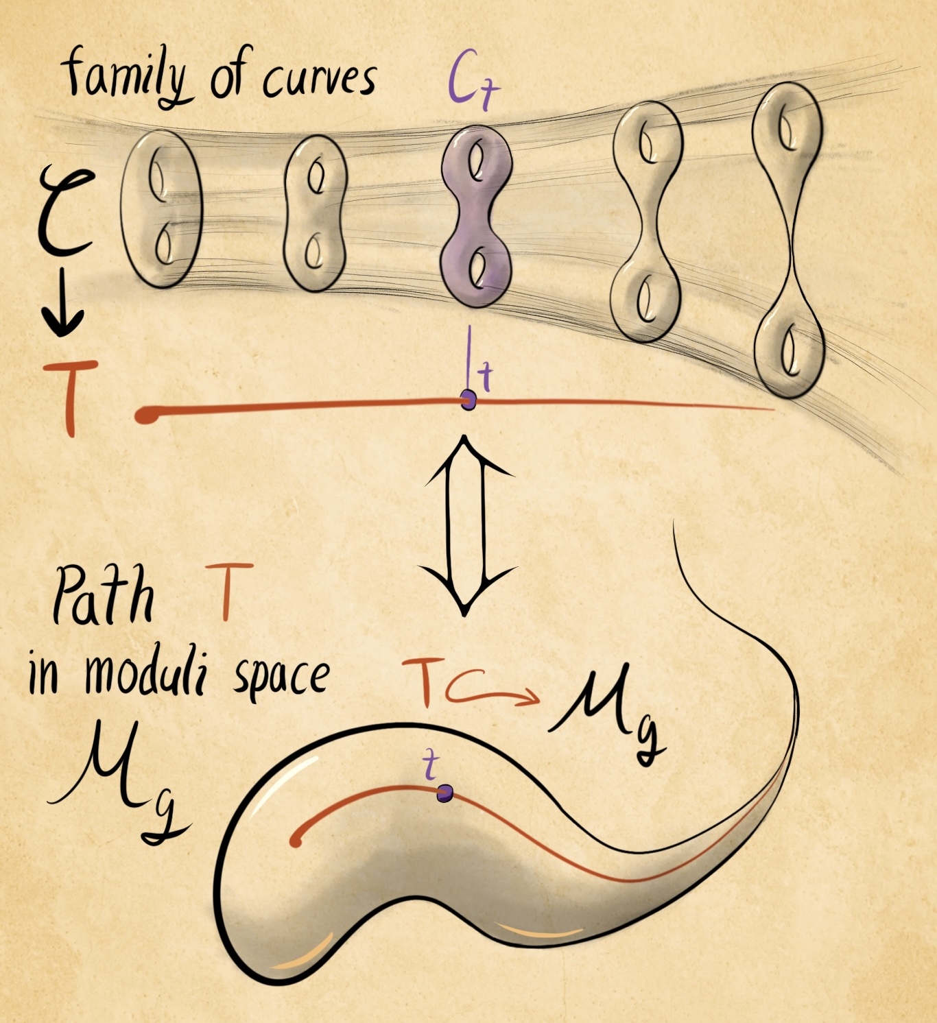
A family of genus g curves over a space $T$ is defined by a map from $T$ into the moduli stack of curves $\mathcal{M}_g$. The picture shows $T$ as a ray, moving off into the cusp of the moduli stack. the associated family of curves pinches into a nodal curve as the ray falls into the cusp.
Stable vs Unstable curves
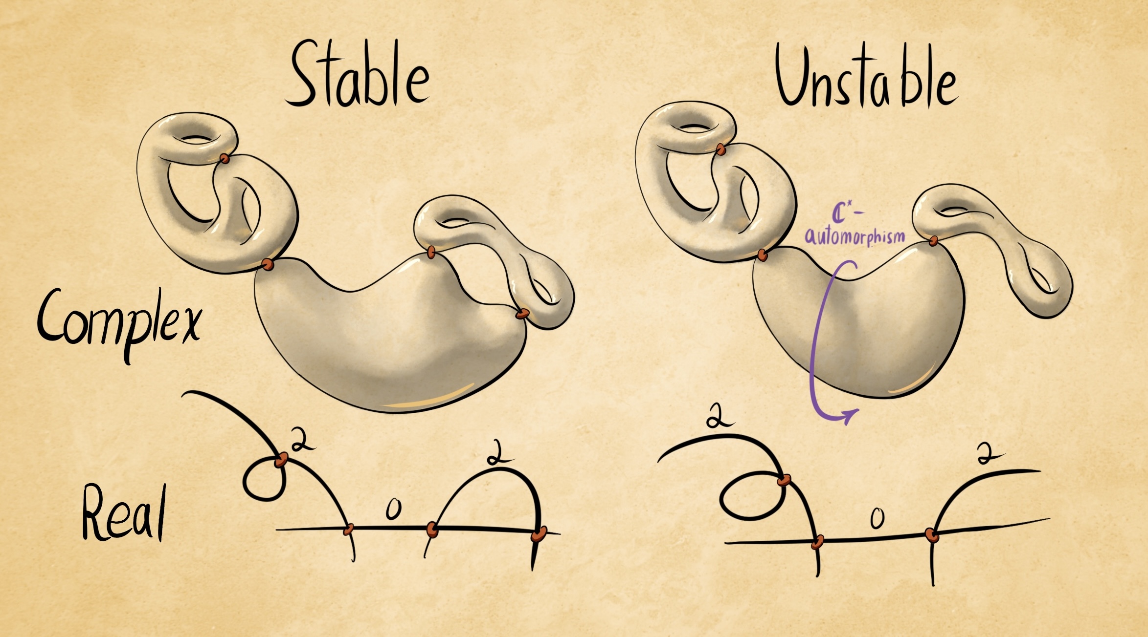
A curve is stable if the space of automorphisms is finite dimensional. It is easy to check stability from a picture of your curve. Every genus 0 component needs at least 3 special points (markings or nodes), and every genus 1 component contains at least 1 special point. The left is an example of a stable curve, and the right an unstable curve. These are rendered both over $\mathbb{R}$ and over $\mathbb{C}$